Summarize participant transitions for a binary longitudinal condition

Create participant-level and condition-level summary tables for a binary condition observed across repeated visits. This function uses the same transition logic and data preparation workflow as PlotSwimmerTransitions() so that plotting and summary outputs remain aligned.

Usage

SummarizeTransitions(
  data,
  id_var,
  time_var,
  status_var,
  date_var = NULL,
  participant_subset = NULL,
  max_participants = NULL,
  order_participants_by = c("first_positive", "first_transition", "ever_positive",
    "ever_positive_then_burden", "input_order", "n_visits", "n_positive", "pct_positive"),
  x_axis_type = c("visit", "date", "time_from_baseline"),
  time_from_baseline_unit = c("days", "months", "years")
)

Arguments

data

A data frame containing repeated observations per participant.

id_var

Unquoted column name identifying the participant.

time_var

Unquoted column name representing visit order, visit number, or time index.

status_var

Unquoted column name representing the binary condition status.

date_var

Optional unquoted visit date column. This is required when x_axis_type = "date" or x_axis_type = "time_from_baseline".

participant_subset

Optional vector of participant IDs to include.

max_participants

Optional maximum number of participants to retain after ordering is applied.

order_participants_by

Character string controlling participant order. Options are "first_positive", "first_transition", "ever_positive", "ever_positive_then_burden", "input_order", "n_visits", "n_positive", and "pct_positive".

x_axis_type

Character string indicating whether longitudinal ordering should follow aligned visit number ("visit"), actual date ("date"), or elapsed time from baseline ("time_from_baseline").

time_from_baseline_unit

Character string specifying the unit for x_axis_type = "time_from_baseline". Options are "days", "months", and "years".

Value

A list with:

• participant_summary: participant-level summary table

• condition_summary: one-row tibble with overall counts

• Plots: figures for the two summaries, described below

Details

Transition rules are:

• 0 -> 1 = developed condition

• 1 -> 0 = resolved condition

Missing values remain missing and are not recoded to 0.

The returned condition-level summary includes:

• number of participants

• number ever positive

• number who developed the condition

• number who resolved the condition

• number sustained after development

• number sustained after resolution

Figures

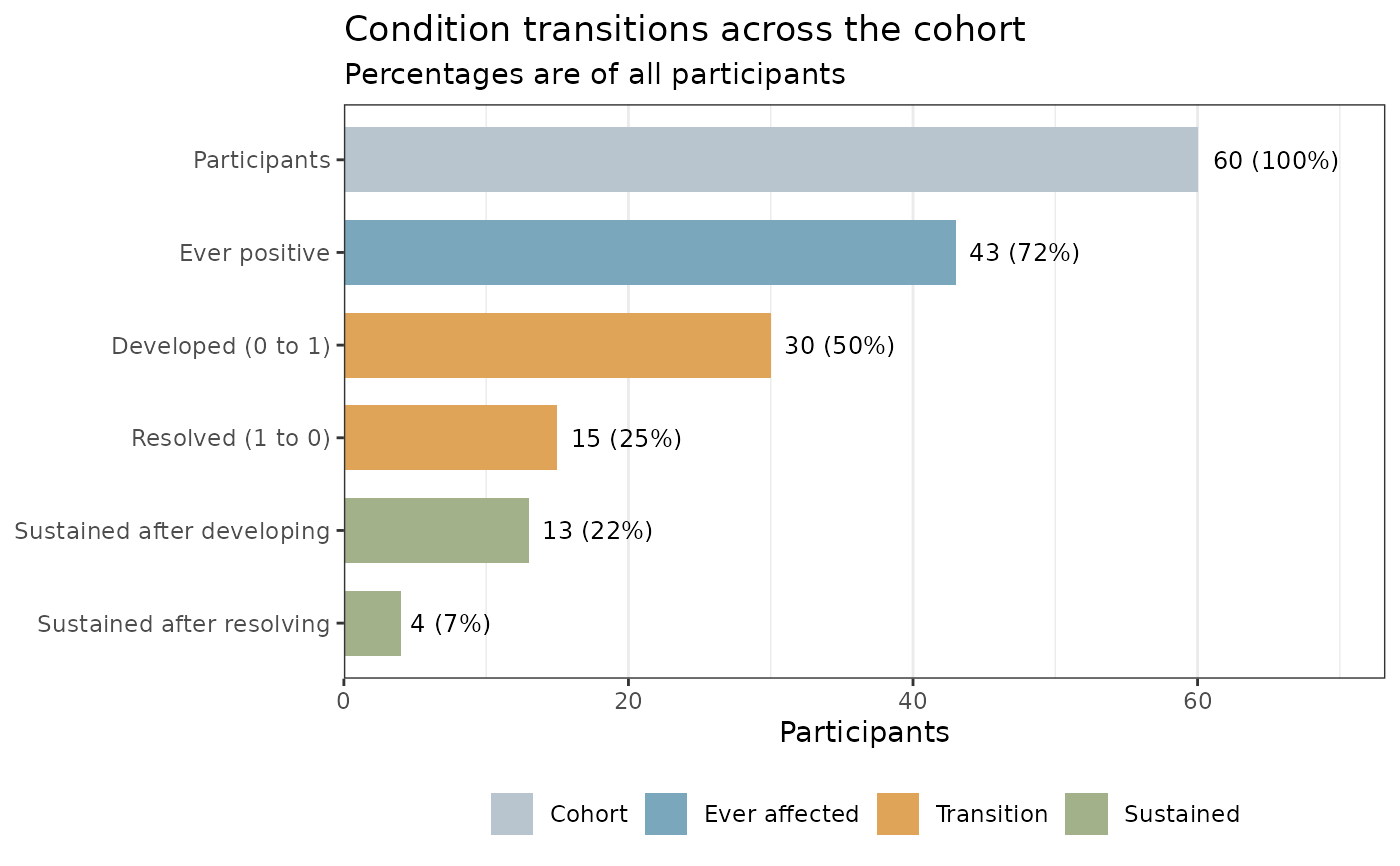
condition_summary is a single row of six counts, which is exactly the shape a table reads worst: the numbers are related to each other, and the relationship is the point. Plots renders them so the relationship is visible:

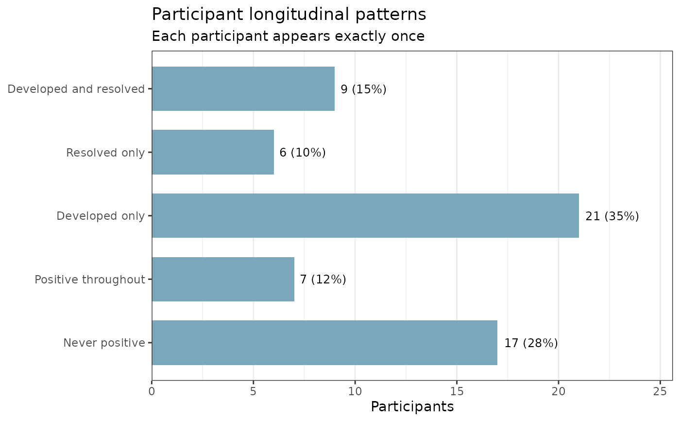
• Plots$ConditionCascade shows the counts as a cascade - the whole cohort, the part of it ever affected, the transitions that occurred within that part, and how many of those persisted - with each bar labelled by its count and its share of the cohort.

• Plots$TransitionPatterns classifies every participant into one mutually exclusive longitudinal pattern (never positive, positive throughout, developed only, resolved only, developed and resolved) and plots the counts. The indicator columns in participant_summary overlap, so this is the view that shows what the cohort is actually made of.

The two agree by construction: the pattern counts sum to n_participants, and everything except "never positive" sums to n_ever_positive.

For the per-participant trajectories behind these counts, use PlotSwimmerTransitions(), which prepares its data the same way.

See also

PlotSwimmerTransitions() for the participant-level swimmer plot.

Examples

toy_df <- tibble::tibble(
  ParticipantID = rep(paste0("P", 1:4), each = 4),
  VisitOrder = rep(1:4, times = 4),
  VisitDate = rep(seq.Date(as.Date("2024-01-01"), by = "month", length.out = 4), times = 4),
  MetSBinary = c(
    0, 0, 1, 1,
    1, 1, 0, 0,
    0, 0, 0, 0,
    TRUE, TRUE, TRUE, TRUE
  )
)

transitions <- SummarizeTransitions(
  data = toy_df,
  id_var = ParticipantID,
  time_var = VisitOrder,
  status_var = MetSBinary,
  date_var = VisitDate,
  x_axis_type = "time_from_baseline",
  time_from_baseline_unit = "months"
)

transitions$condition_summary
#> # A tibble: 1 × 6
#>   n_participants n_ever_positive n_developed_condition n_resolved_condition
#>            <int>           <int>                 <int>                <int>
#> 1              4               3                     1                    1
#> # ℹ 2 more variables: n_sustained_after_development <int>,
#> #   n_sustained_after_resolution <int>

# \donttest{
# A larger cohort, where a positive visit tends to be followed by another
set.seed(9)
n_participants <- 60

df_Longitudinal <- do.call(rbind, lapply(seq_len(n_participants), function(i) {
  n_visits <- sample(3:5, 1)
  status <- numeric(n_visits)
  status[1] <- stats::rbinom(1, 1, 0.3)
  for (j in seq_len(n_visits)[-1]) {
    status[j] <- stats::rbinom(1, 1, if (status[j - 1] == 1) 0.8 else 0.25)
  }
  data.frame(
    ParticipantID = sprintf("P%02d", i),
    VisitOrder = seq_len(n_visits),
    MetSBinary = status
  )
}))

transitions <- SummarizeTransitions(
  data = df_Longitudinal,
  id_var = ParticipantID,
  time_var = VisitOrder,
  status_var = MetSBinary
)

# Six counts in one row
htmltools::browsable(htmltools::HTML(as.character(
  FreezeTableHeader(transitions$condition_summary, full_width = TRUE)
)))
 n_participants 
   
 n_ever_positive 
   
 n_developed_condition 
   
 n_resolved_condition 
   
 n_sustained_after_development 
   
 n_sustained_after_resolution 
  
 60 
   
 43 
   
 30 
   
 15 
   
 13 
   
 4 
  

# The same six numbers as a cascade
transitions$Plots$ConditionCascade


# The cohort split into mutually exclusive patterns
transitions$Plots$TransitionPatterns


# The participant-level table
htmltools::browsable(htmltools::HTML(as.character(
  FreezeTableHeader(
    dplyr::select(
      transitions$participant_summary,
      .plot_id, n_visits, n_positive, pct_positive, ever_positive,
      developed_condition, resolved_condition
    ),
    height = "300px", full_width = TRUE
  )
)))
 .plot_id 
   
 n_visits 
   
 n_positive 
   
 pct_positive 
   
 ever_positive 
   
 developed_condition 
   
 resolved_condition 
  
 P06 
   
 4 
   
 2 
   
 0.5000000 
   
 TRUE 
   
 TRUE 
   
 TRUE 
  
 P07 
   
 4 
   
 3 
   
 0.7500000 
   
 TRUE 
   
 TRUE 
   
 TRUE 
  
 P10 
   
 5 
   
 2 
   
 0.4000000 
   
 TRUE 
   
 TRUE 
   
 TRUE 
  
 P11 
   
 4 
   
 4 
   
 1.0000000 
   
 TRUE 
   
 FALSE 
   
 FALSE 
  
 P13 
   
 5 
   
 5 
   
 1.0000000 
   
 TRUE 
   
 FALSE 
   
 FALSE 
  
 P19 
   
 5 
   
 5 
   
 1.0000000 
   
 TRUE 
   
 FALSE 
   
 FALSE 
  
 P20 
   
 5 
   
 5 
   
 1.0000000 
   
 TRUE 
   
 FALSE 
   
 FALSE 
  
 P26 
   
 3 
   
 3 
   
 1.0000000 
   
 TRUE 
   
 FALSE 
   
 FALSE 
  
 P27 
   
 4 
   
 3 
   
 0.7500000 
   
 TRUE 
   
 FALSE 
   
 TRUE 
  
 P30 
   
 5 
   
 3 
   
 0.6000000 
   
 TRUE 
   
 TRUE 
   
 TRUE 
  
 P32 
   
 4 
   
 3 
   
 0.7500000 
   
 TRUE 
   
 TRUE 
   
 TRUE 
  
 P43 
   
 3 
   
 2 
   
 0.6666667 
   
 TRUE 
   
 FALSE 
   
 TRUE 
  
 P44 
   
 5 
   
 2 
   
 0.4000000 
   
 TRUE 
   
 FALSE 
   
 TRUE 
  
 P49 
   
 3 
   
 3 
   
 1.0000000 
   
 TRUE 
   
 FALSE 
   
 FALSE 
  
 P53 
   
 4 
   
 1 
   
 0.2500000 
   
 TRUE 
   
 FALSE 
   
 TRUE 
  
 P56 
   
 5 
   
 3 
   
 0.6000000 
   
 TRUE 
   
 FALSE 
   
 TRUE 
  
 P58 
   
 3 
   
 3 
   
 1.0000000 
   
 TRUE 
   
 FALSE 
   
 FALSE 
  
 P60 
   
 3 
   
 2 
   
 0.6666667 
   
 TRUE 
   
 FALSE 
   
 TRUE 
  
 P05 
   
 3 
   
 2 
   
 0.6666667 
   
 TRUE 
   
 TRUE 
   
 FALSE 
  
 P08 
   
 3 
   
 1 
   
 0.3333333 
   
 TRUE 
   
 TRUE 
   
 TRUE 
  
 P23 
   
 4 
   
 3 
   
 0.7500000 
   
 TRUE 
   
 TRUE 
   
 FALSE 
  
 P24 
   
 4 
   
 3 
   
 0.7500000 
   
 TRUE 
   
 TRUE 
   
 FALSE 
  
 P36 
   
 5 
   
 4 
   
 0.8000000 
   
 TRUE 
   
 TRUE 
   
 FALSE 
  
 P39 
   
 5 
   
 4 
   
 0.8000000 
   
 TRUE 
   
 TRUE 
   
 FALSE 
  
 P42 
   
 4 
   
 3 
   
 0.7500000 
   
 TRUE 
   
 TRUE 
   
 FALSE 
  
 P50 
   
 5 
   
 1 
   
 0.2000000 
   
 TRUE 
   
 TRUE 
   
 TRUE 
  
 P02 
   
 5 
   
 3 
   
 0.6000000 
   
 TRUE 
   
 TRUE 
   
 FALSE 
  
 P04 
   
 5 
   
 3 
   
 0.6000000 
   
 TRUE 
   
 TRUE 
   
 FALSE 
  
 P29 
   
 3 
   
 1 
   
 0.3333333 
   
 TRUE 
   
 TRUE 
   
 FALSE 
  
 P38 
   
 4 
   
 1 
   
 0.2500000 
   
 TRUE 
   
 TRUE 
   
 TRUE 
  
 P46 
   
 4 
   
 1 
   
 0.2500000 
   
 TRUE 
   
 TRUE 
   
 TRUE 
  
 P51 
   
 5 
   
 3 
   
 0.6000000 
   
 TRUE 
   
 TRUE 
   
 FALSE 
  
 P15 
   
 5 
   
 2 
   
 0.4000000 
   
 TRUE 
   
 TRUE 
   
 FALSE 
  
 P18 
   
 4 
   
 1 
   
 0.2500000 
   
 TRUE 
   
 TRUE 
   
 FALSE 
  
 P34 
   
 4 
   
 1 
   
 0.2500000 
   
 TRUE 
   
 TRUE 
   
 FALSE 
  
 P37 
   
 5 
   
 2 
   
 0.4000000 
   
 TRUE 
   
 TRUE 
   
 FALSE 
  
 P45 
   
 5 
   
 2 
   
 0.4000000 
   
 TRUE 
   
 TRUE 
   
 FALSE 
  
 P47 
   
 5 
   
 2 
   
 0.4000000 
   
 TRUE 
   
 TRUE 
   
 FALSE 
  
 P54 
   
 4 
   
 1 
   
 0.2500000 
   
 TRUE 
   
 TRUE 
   
 FALSE 
  
 P09 
   
 5 
   
 1 
   
 0.2000000 
   
 TRUE 
   
 TRUE 
   
 FALSE 
  
 P17 
   
 5 
   
 1 
   
 0.2000000 
   
 TRUE 
   
 TRUE 
   
 FALSE 
  
 P33 
   
 5 
   
 1 
   
 0.2000000 
   
 TRUE 
   
 TRUE 
   
 FALSE 
  
 P52 
   
 5 
   
 1 
   
 0.2000000 
   
 TRUE 
   
 TRUE 
   
 FALSE 
  
 P01 
   
 5 
   
 0 
   
 0.0000000 
   
 FALSE 
   
 FALSE 
   
 FALSE 
  
 P03 
   
 3 
   
 0 
   
 0.0000000 
   
 FALSE 
   
 FALSE 
   
 FALSE 
  
 P12 
   
 3 
   
 0 
   
 0.0000000 
   
 FALSE 
   
 FALSE 
   
 FALSE 
  
 P14 
   
 3 
   
 0 
   
 0.0000000 
   
 FALSE 
   
 FALSE 
   
 FALSE 
  
 P16 
   
 3 
   
 0 
   
 0.0000000 
   
 FALSE 
   
 FALSE 
   
 FALSE 
  
 P21 
   
 3 
   
 0 
   
 0.0000000 
   
 FALSE 
   
 FALSE 
   
 FALSE 
  
 P22 
   
 5 
   
 0 
   
 0.0000000 
   
 FALSE 
   
 FALSE 
   
 FALSE 
  
 P25 
   
 3 
   
 0 
   
 0.0000000 
   
 FALSE 
   
 FALSE 
   
 FALSE 
  
 P28 
   
 3 
   
 0 
   
 0.0000000 
   
 FALSE 
   
 FALSE 
   
 FALSE 
  
 P31 
   
 4 
   
 0 
   
 0.0000000 
   
 FALSE 
   
 FALSE 
   
 FALSE 
  
 P35 
   
 4 
   
 0 
   
 0.0000000 
   
 FALSE 
   
 FALSE 
   
 FALSE 
  
 P40 
   
 4 
   
 0 
   
 0.0000000 
   
 FALSE 
   
 FALSE 
   
 FALSE 
  
 P41 
   
 4 
   
 0 
   
 0.0000000 
   
 FALSE 
   
 FALSE 
   
 FALSE 
  
 P48 
   
 3 
   
 0 
   
 0.0000000 
   
 FALSE 
   
 FALSE 
   
 FALSE 
  
 P55 
   
 3 
   
 0 
   
 0.0000000 
   
 FALSE 
   
 FALSE 
   
 FALSE 
  
 P57 
   
 4 
   
 0 
   
 0.0000000 
   
 FALSE 
   
 FALSE 
   
 FALSE 
  
 P59 
   
 4 
   
 0 
   
 0.0000000 
   
 FALSE 
   
 FALSE 
   
 FALSE 
  
# }