Apply a normative T-score model to new data

Applies a previously fitted normative regression model to new data and computes predicted values, z-scores, and T-scores using the same preprocessing settings used during model development.

Usage

ApplyNormativeTScores(
  data,
  normative_obj,
  score_prefix = "Norm",
  df = lifecycle::deprecated()
)

Arguments

data

A data frame containing the test variable, count variable, and all predictors required by the normative model.

normative_obj

A list returned by CreateNormativeTScoreModel().

score_prefix

A character string prefix used when naming output columns. Defaults to "Norm".

df

Deprecated (since 19.15.0). Use data instead.

Value

A tibble containing the original data plus scored columns, each named using the score_prefix string as a prefix:

{score_prefix}Raw

The raw input score.

{score_prefix}Scaled

The transformed analysis-scale score.

{score_prefix}Predicted

The predicted score from the normative model.

{score_prefix}Z

The z-score.

{score_prefix}T

The T-score.

Details

This function is designed to work with the output of CreateNormativeTScoreModel(). It uses the saved model and preprocessing settings to score new observations consistently.

What the example shows

The example builds a cohort with a healthy reference group and a clinical group tested on Trail Making A. Times are recorded in milliseconds, get slower with age, and improve a little each time the test is repeated. The norms are fitted on the reference group only, adjusting for demographics and for practice across visits, and then everyone is scored through that same model.

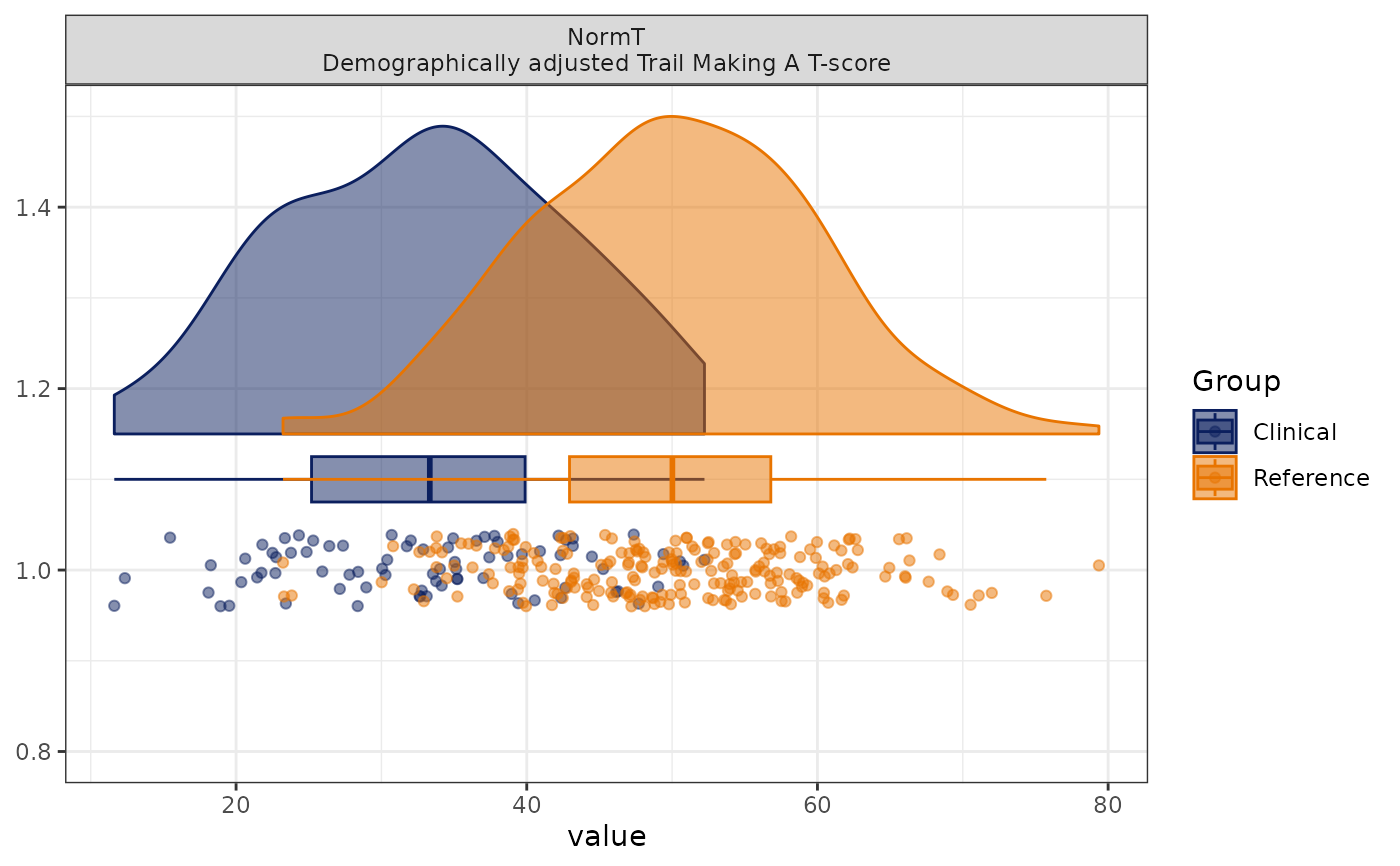
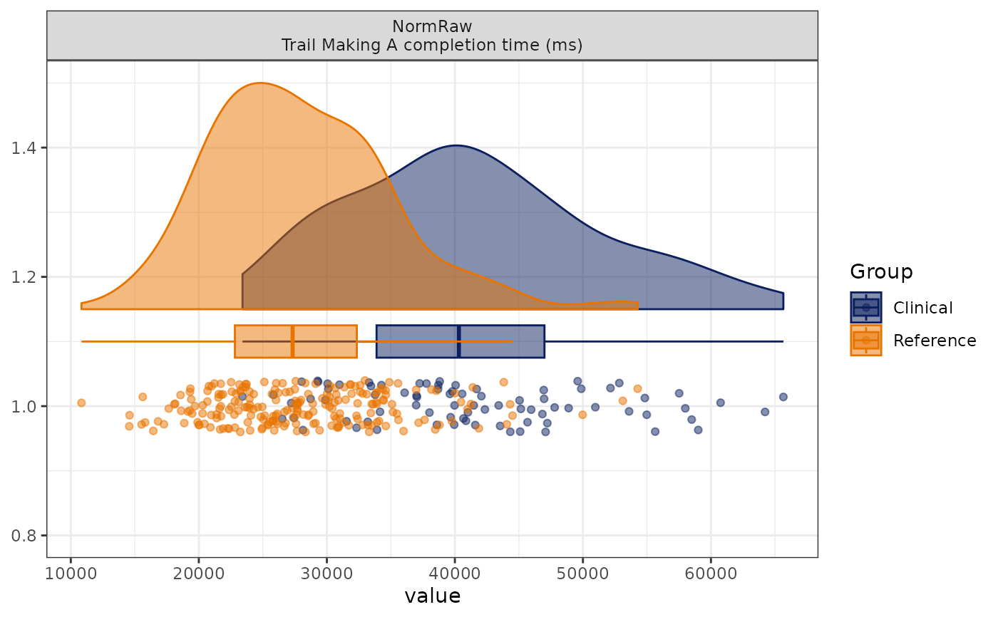
The two density plots are the payoff. Raw completion times are right-skewed and in test-specific units, and whether 40 seconds is unusual depends on who the participant is, so the groups are hard to compare by eye. T-scores put everyone on one interpretable scale: the reference group is centered at 50 with a standard deviation of 10 by construction, so the clinical group's shift can be read straight off the axis - here about 1.7 SD below expectation for their age, education, sex, and visit number.

Examples

# A reference group and a clinical group tested on Trail Making A
set.seed(206)
n_reference <- 220
n_clinical <- 80

df <- tibble::tibble(
  Group = c(rep("Reference", n_reference), rep("Clinical", n_clinical)),
  Age = round(c(
    stats::rnorm(n_reference, 52, 12),
    stats::rnorm(n_clinical, 58, 12)
  )),
  Education = factor(sample(
    c("HighSchool", "College", "Graduate"), n_reference + n_clinical,
    replace = TRUE
  )),
  Sex = factor(sample(c("F", "M"), n_reference + n_clinical, replace = TRUE)),
  Visit = sample(1:3, n_reference + n_clinical, replace = TRUE)
)
df$TrailsA <- round(1000 * exp(stats::rnorm(
  nrow(df),
  mean = log(28) + 0.011 * (df$Age - 52) - 0.05 * (df$Visit - 1) +
    ifelse(df$Group == "Clinical", 0.35, 0),
  sd = 0.22
)))

# Fit the norms on the reference group only
norm_obj <- CreateNormativeTScoreModel(
  data = df,
  test_var = "TrailsA",
  count_var = "Visit",
  covariates = c("Age", "Education", "Sex"),
  reference_var = "Group",
  reference_value = "Reference",
  include_practice_effect = TRUE,
  reverse_score = TRUE,
  convert_seconds = TRUE,
  log_transform = TRUE,
  return_plots = FALSE
)

# Score everyone through the same model
scored_df <- ApplyNormativeTScores(
  data = df,
  normative_obj = norm_obj
)

# Before: raw completion times, grouped by clinical status
attr(scored_df$NormRaw, "label") <- "Trail Making A completion time (ms)"
PlotContinuousDistributions(
  scored_df, variables = "NormRaw", Fill = "Group", ncol = 1
)
#> Registered S3 methods overwritten by 'ggpp':
#>   method                  from   
#>   heightDetails.titleGrob ggplot2
#>   widthDetails.titleGrob  ggplot2


# After: demographically adjusted T-scores. The reference group is centered
# near 50, and the clinical shift is now directly interpretable in SD units.
attr(scored_df$NormT, "label") <- "Demographically adjusted Trail Making A T-score"
PlotContinuousDistributions(
  scored_df, variables = "NormT", Fill = "Group", ncol = 1
)