Exploring associations with PlotCorrelationsHeatmap()

1 Overview

PlotCorrelationsHeatmap() computes correlations or partial correlations and visualizes the results as a heatmap.

This vignette demonstrates:

Correlations among biomarkers
Correlations between biomarkers and clinical variables
Pearson versus Spearman correlations
False discovery rate (FDR) correction
Covariate-adjusted correlations
Annotating heatmaps with correlation coefficients and significance stars
Interactive exploration using plotly
Follow-up visualization of significant correlations

2 Load packages

library(SciDataReportR)
library(dplyr)
library(plotly)

3 Load example data

SciDataReportR includes an example dataset and variable type specification file.

data("SampleData")
data("SampleVariableTypes")

RevaluedObj <- RevalueData(
  SampleData,
  SampleVariableTypes
)

df_Revalued <- RevaluedObj$RevaluedData

4 Select biomarkers

For this vignette we will examine relationships among a panel of biomarkers.

biomarkers <- c(
  "AXL",
  "Calbindin",
  "Ferritin",
  "MMP7",
  "MMP10",
  "NFL",
  "GFAP",
  "IL6",
  "VCAM1",
  "ICAM1",
  "CRP",
  "TNFa",
  "MCP1",
  "YKL40",
  "Tau"
)

5 Correlations among biomarkers

When only xVars are supplied, a square correlation matrix is generated.

CorrObj <- PlotCorrelationsHeatmap(
  Data = df_Revalued,
  xVars = biomarkers
)

CorrObj$Unadjusted$plot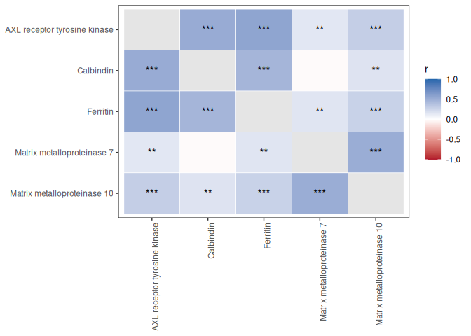

Each tile represents the correlation coefficient between two biomarkers. Positive and negative correlations are represented by opposite ends of the color scale.

6 Correlations between biomarkers and clinical variables

A rectangular correlation matrix can be created by supplying both xVars and yVars.

clinical_vars <- c(
  "age",
  "Insulin"
)

CorrObj_Clinical <- PlotCorrelationsHeatmap(
  Data = df_Revalued,
  xVars = biomarkers,
  yVars = clinical_vars
)

CorrObj_Clinical$Unadjusted$plot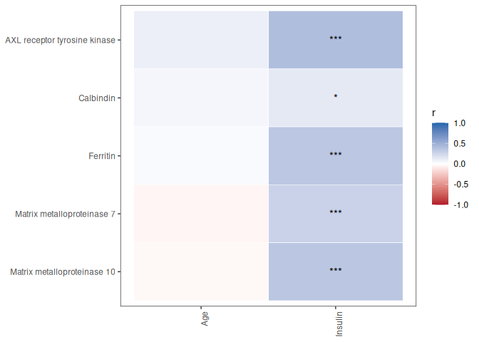

This approach is useful for screening biomarker-clinical relationships.

7 Pearson versus Spearman correlations

The choice of correlation method depends on the characteristics of the data.

Method	Recommended Use
Pearson	Approximately normal variables with linear relationships
Spearman	Skewed variables, outliers, or monotonic relationships
Kendall	Small samples or ordinal variables

7.1 Pearson correlations

Pearson correlation measures linear relationships between variables and is most appropriate when variables are approximately normally distributed.

PearsonObj <- PlotCorrelationsHeatmap(
  Data = df_Revalued,
  xVars = biomarkers,
  method = "pearson"
)

PearsonObj$Unadjusted$plot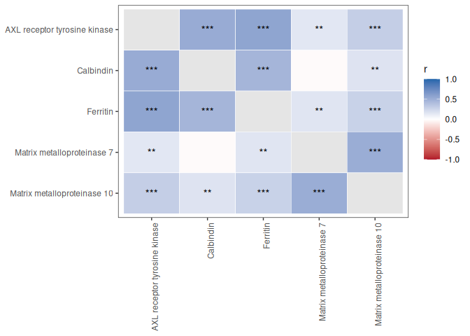

7.2 Spearman correlations

Spearman correlation is rank-based and is often preferred for biomarker data because it is more robust to skewed distributions and outliers.

SpearmanObj <- PlotCorrelationsHeatmap(
  Data = df_Revalued,
  xVars = biomarkers,
  method = "spearman"
)

SpearmanObj$Unadjusted$plot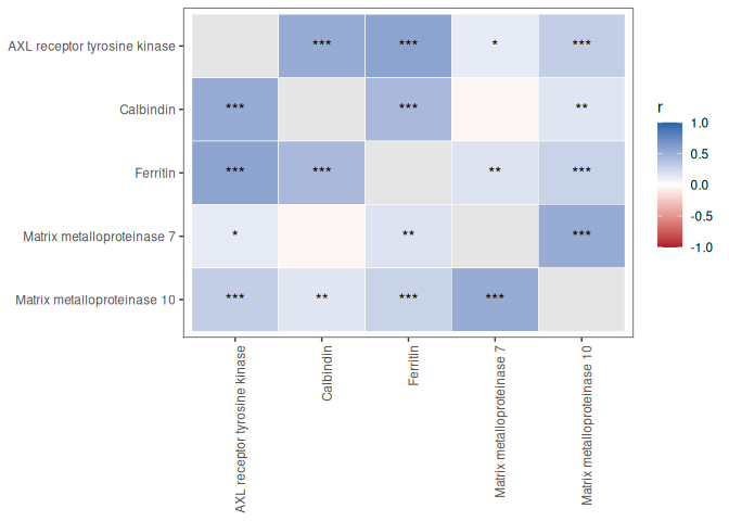

Researchers frequently compare both methods to determine whether findings are sensitive to distributional assumptions.

8 Unadjusted versus FDR-corrected significance

PlotCorrelationsHeatmap() automatically computes both unadjusted and FDR-corrected p-values.

8.1 Unadjusted significance

CorrObj$Unadjusted$plot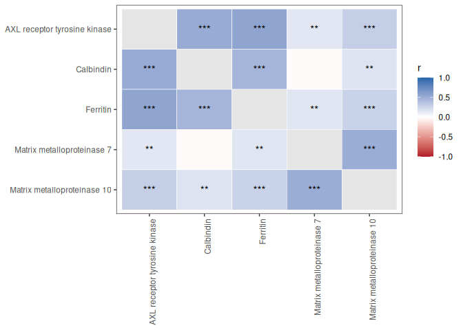

8.2 FDR-corrected significance

CorrObj$FDRCorrected$plot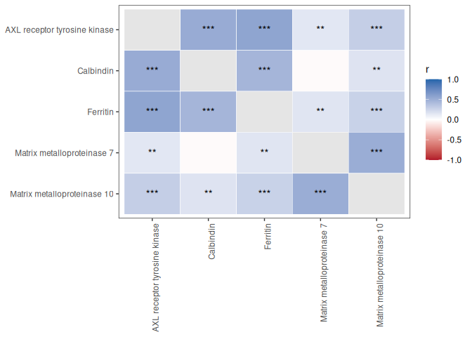

When evaluating many correlations simultaneously, false discovery rate correction is recommended to reduce the likelihood of false positive findings.

9 Adding correlation coefficients and significance stars

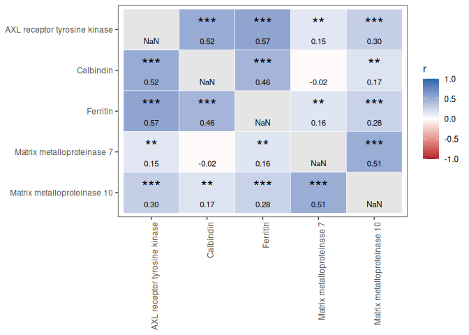
The default heatmaps display significance stars. Additional annotations can be added using add_r_and_stars().

9.1 Raw p-values

add_r_and_stars(
  CorrObj,
  star_from = "raw"
)

9.2 FDR-corrected p-values

add_r_and_stars(
  CorrObj,
  star_from = "fdr"
)

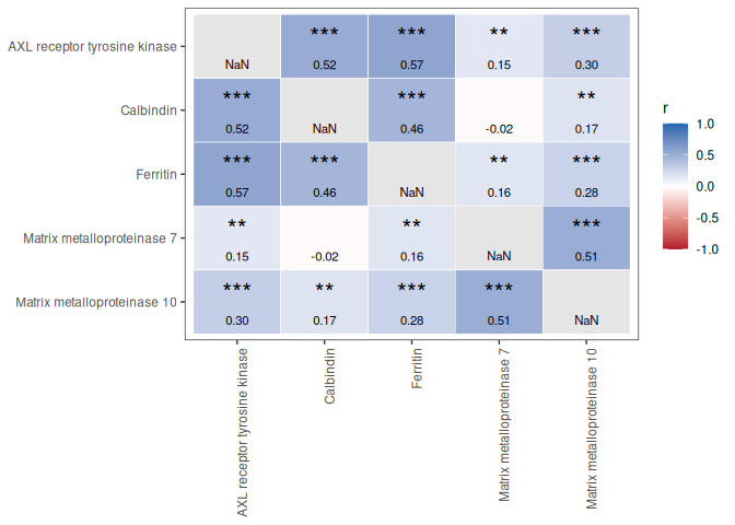
These annotated heatmaps are useful for presentations and publications.

10 Adjusting for covariates

Partial correlations can be estimated by specifying one or more covariates.

The example below adjusts all correlations for age.

CorrObj_AgeAdjusted <- PlotCorrelationsHeatmap(
  Data = df_Revalued,
  xVars = biomarkers,
  covars = "age"
)

CorrObj_AgeAdjusted$FDRCorrected$plot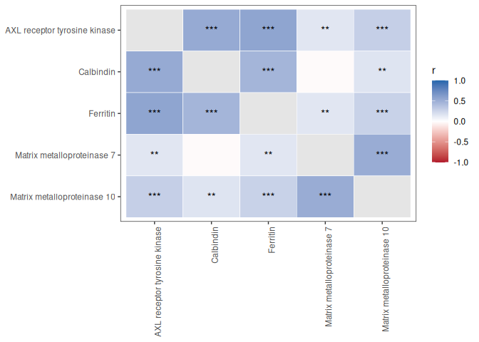

When covariates are supplied, variables are residualized prior to correlation testing. This can help account for potential confounding factors.

11 Interactive heatmaps

Heatmaps can be converted into interactive visualizations using plotly.

# Not evaluated in the shipped vignette to keep it lightweight - run interactively
ggplotly(
  CorrObj$FDRCorrected$plot
)

Interactive plots allow users to:

Hover over cells to inspect values
Zoom into regions of interest
Explore large correlation matrices

12 Investigating significant correlations

Significant correlations can be examined individually using plotSigCorrelations().

SigPlots <- plotSigCorrelations(
  DataFrame = df_Revalued,
  CorrelationHeatmapObject = CorrObj
)

The resulting object contains a list of scatterplots for significant associations, one per significant heatmap cell.

length(SigPlots)

These plots can be combined into a single figure.

AssemblePlots(
  SigPlots,
  LegendPosition = "none",
  ncol = 3
)

These plotSigCorrelations() / AssemblePlots() chunks are shown but not executed when the vignette is built, because the underlying ggstatsplot scatterplots require graphics fonts that are not available on all systems. Run them interactively to reproduce the figures.

This workflow provides a convenient way to visually inspect the relationships underlying significant heatmap cells.

13 Accessing correlation results

The returned object stores both correlation estimates and p-values.

13.1 Unadjusted results

head(
  CorrObj$Unadjusted$r
)

                AXL   Calbindin  Ferritin        MMP7     MMP10
AXL             NaN  0.52216065 0.5653655  0.14869241 0.3022935
Calbindin 0.5221607         NaN 0.4583562 -0.02312424 0.1680769
Ferritin  0.5653655  0.45835621       NaN  0.15786447 0.2789080
MMP7      0.1486924 -0.02312424 0.1578645         NaN 0.5129789
MMP10     0.3022935  0.16807693 0.2789080  0.51297885       NaN

13.2 FDR-corrected results

head(
  CorrObj$FDRCorrected$p
)

                   AXL    Calbindin     Ferritin         MMP7        MMP10
AXL                 NA 5.467874e-24 1.603627e-28 7.290795e-03 3.650376e-08
Calbindin 5.467874e-24           NA 2.646785e-18 6.741588e-01 2.982019e-03
Ferritin  1.603627e-28 2.646785e-18           NA 4.845409e-03 3.829675e-07
MMP7      7.290795e-03 6.741588e-01 4.845409e-03           NA 3.179809e-23
MMP10     3.650376e-08 2.982019e-03 3.829675e-07 3.179809e-23           NA

These results can be exported for reporting or used in downstream analyses.

14 Summary

PlotCorrelationsHeatmap() provides a comprehensive workflow for exploratory association analysis, including:

Pearson, Spearman, and Kendall correlations
Partial correlations using covariate adjustment
Automatic FDR correction
Label-aware visualization
Interactive heatmaps
Correlation coefficient annotation
Follow-up visualization of significant associations

16 Session information

sessionInfo()

R version 4.6.1 (2026-06-24)
Platform: x86_64-pc-linux-gnu
Running under: Ubuntu 24.04.4 LTS

Matrix products: default
BLAS:   /usr/lib/x86_64-linux-gnu/openblas-pthread/libblas.so.3
LAPACK: /usr/lib/x86_64-linux-gnu/openblas-pthread/libopenblasp-r0.3.26.so;  LAPACK version 3.12.0

locale:
 [1] LC_CTYPE=C.UTF-8       LC_NUMERIC=C           LC_TIME=C.UTF-8
 [4] LC_COLLATE=C.UTF-8     LC_MONETARY=C.UTF-8    LC_MESSAGES=C.UTF-8
 [7] LC_PAPER=C.UTF-8       LC_NAME=C              LC_ADDRESS=C
[10] LC_TELEPHONE=C         LC_MEASUREMENT=C.UTF-8 LC_IDENTIFICATION=C

time zone: UTC
tzcode source: system (glibc)

attached base packages:
[1] stats     graphics  grDevices utils     datasets  methods   base

other attached packages:
[1] plotly_4.12.0         ggplot2_4.0.3         dplyr_1.2.1
[4] SciDataReportR_20.9.0

loaded via a namespace (and not attached):
 [1] gtable_0.3.6           xfun_0.59              bayestestR_0.18.1
 [4] htmlwidgets_1.6.4      insight_1.5.2          rstatix_1.0.0
 [7] lattice_0.22-9         paletteer_1.7.0        vctrs_0.7.3
[10] tools_4.6.1            generics_0.1.4         datawizard_1.3.1
[13] tibble_3.3.1           pkgconfig_2.0.3        data.table_1.18.4
[16] RColorBrewer_1.1-3     correlation_0.8.8      S7_0.2.2
[19] RcppParallel_5.1.11-2  lifecycle_1.0.5        compiler_4.6.1
[22] farver_2.1.2           snakecase_0.11.1       carData_3.0-6
[25] htmltools_0.5.9        lazyeval_0.2.3         yaml_2.3.12
[28] Formula_1.2-5          pillar_1.11.1          car_3.1-5
[31] tidyr_1.3.2            broom.helpers_1.22.0   statsExpressions_2.0.0
[34] abind_1.4-8            tidyselect_1.2.1       sjlabelled_1.2.0
[37] digest_0.6.39          mvtnorm_1.4-1          gtsummary_2.5.1
[40] purrr_1.2.2            rematch2_2.1.2         labeling_0.4.3
[43] forcats_1.0.1          ggstatsplot_1.0.0      labelled_2.16.0
[46] fastmap_1.2.0          grid_4.6.1             cli_3.6.6
[49] magrittr_2.0.5         patchwork_1.3.2        dichromat_2.0-0.1
[52] broom_1.0.13           withr_3.0.3            scales_1.4.0
[55] backports_1.5.1        estimability_2.0.0     httr_1.4.8
[58] rmarkdown_2.31         emmeans_2.0.3          otel_0.2.0
[61] hms_1.1.4              coda_0.19-4.1          evaluate_1.0.5
[64] knitr_1.51             haven_2.5.5            parameters_0.29.2
[67] viridisLite_0.4.3      rstantools_2.6.0       rlang_1.2.0
[70] xtable_1.8-8           glue_1.8.1             jsonlite_2.0.0
[73] effectsize_1.0.2       R6_2.6.1