Exploratory discovery with PlotMiningMatrix()

1 Overview

PlotMiningMatrix() is designed for exploratory data mining and hypothesis generation.

Rather than requiring separate correlation analyses, ANOVA models, and chi-square tests, the function automatically identifies appropriate statistical relationships based on variable type and summarizes the results in a single visualization.

This function is particularly useful for:

Identifying unexpected relationships
Detecting potential confounders and covariates
Discovering clusters of related variables
Generating hypotheses for future analyses
Performing exploratory quality control
Prioritizing variables for downstream modeling

Unlike a traditional correlation matrix, PlotMiningMatrix() can simultaneously evaluate:

Continuous vs continuous relationships
Categorical vs continuous relationships
Categorical vs categorical relationships

using appropriate statistical methods for each comparison.

2 Load packages

library(SciDataReportR)
library(dplyr)
library(plotly)

3 Load example data

data("SampleData")
data("SampleVariableTypes")

RevaluedObj <- RevalueData(
  SampleData,
  SampleVariableTypes
)

df_Revalued <- RevaluedObj$RevaluedData

4 Create a mining matrix

For exploratory mining it is often useful to evaluate nearly the entire dataset simultaneously.

vars_mining <- names(df_Revalued)

length(vars_mining)

[1] 131

MiningObj <- PlotMiningMatrix(
  Data = df_Revalued,
  OutcomeVars = vars_mining
)

MiningObj$Unadjusted$plot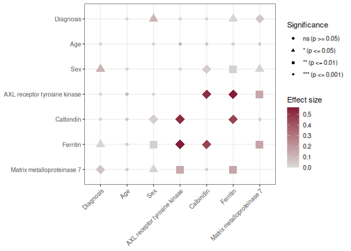

The resulting visualization summarizes hundreds or thousands of statistical relationships simultaneously.

Color intensity represents effect size magnitude, while symbol size and shape represent statistical significance.

5 Understanding the statistical tests

PlotMiningMatrix() automatically selects appropriate analyses based on variable type.

Variable Types	Statistical Test
Continuous vs Continuous	Correlation
Categorical vs Continuous	ANOVA
Categorical vs Categorical	Chi-square

This allows mixed datasets to be explored without manually specifying separate analyses.

6 Interpreting the mining matrix

The mining matrix is best viewed as a discovery tool rather than a confirmatory analysis.

Questions it can help answer include:

Which biomarkers appear related to diagnosis?
Which demographic variables may act as covariates?
Which variables tend to cluster together?
Are there unexpected associations worth investigating?
Are there patterns suggesting data quality issues?

Large effect sizes combined with strong significance often represent promising targets for follow-up analyses.

7 Parametric analyses

By default, parametric analyses are used.

MiningParametric <- PlotMiningMatrix(
  Data = df_Revalued,
  OutcomeVars = vars_mining,
  Parametric = TRUE
)

MiningParametric$Unadjusted$plot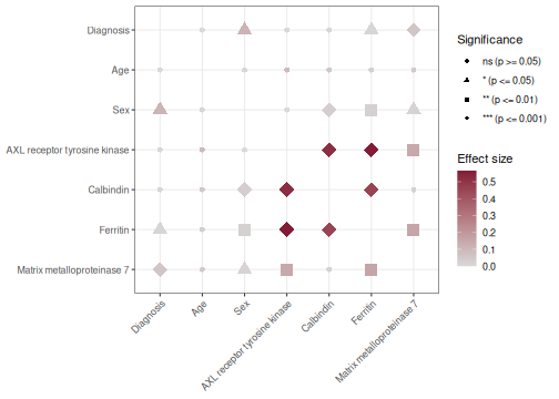

For continuous variables this uses Pearson correlations and parametric group comparisons.

8 Nonparametric analyses

For skewed variables or datasets containing substantial outliers, nonparametric methods may be preferable.

MiningNonParametric <- PlotMiningMatrix(
  Data = df_Revalued,
  OutcomeVars = vars_mining,
  Parametric = FALSE
)

MiningNonParametric$Unadjusted$plot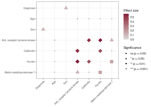

This switches continuous-variable analyses to Spearman correlations and uses nonparametric group comparisons where applicable.

9 Unadjusted significance

The default plot displays significance based on unadjusted p-values.

MiningObj$Unadjusted$plot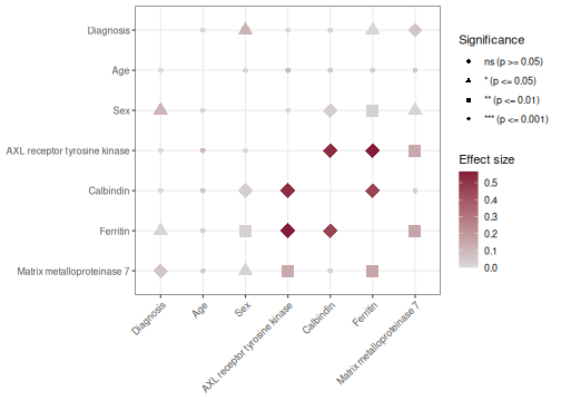

This view is useful for exploratory analyses and hypothesis generation.

10 FDR-corrected significance

Because large mining matrices may involve hundreds or thousands of statistical tests, multiple-testing correction is often recommended.

MiningObj$FDRCorrected$plot

NULL

The FDR-corrected visualization highlights relationships that remain significant after accounting for multiple comparisons.

In exploratory studies, investigators often review both unadjusted and FDR-corrected results.

11 Examining the underlying results

The statistical results are stored in the returned object.

head(
  MiningObj$Unadjusted$PvalTable
)

# A tibble: 6 × 11
  XVar              YVar         p EffectSize Test     p_adj stars XLabel YLabel
  <chr>             <chr>    <dbl>      <dbl> <chr>    <dbl> <chr> <fct>  <fct>
1 ACE_CD143_Angiot… ACTH… 4.03e- 8     0.295  Corr… 1.30e- 7 ****  Angio… Adren…
2 ACE_CD143_Angiot… AXL   2.32e-51     0.705  Corr… 1.90e-49 ****  Angio… AXL r…
3 ACE_CD143_Angiot… Adip… 1.40e- 1     0.0811 Corr… 1.89e- 1 ns    Angio… Adipo…
4 ACE_CD143_Angiot… Alph… 2.13e- 5     0.231  Corr… 5.24e- 5 ****  Angio… Alpha…
5 ACE_CD143_Angiot… Alph… 4.69e- 1     0.0399 Corr… 5.39e- 1 ns    Angio… Alpha…
6 ACE_CD143_Angiot… Alph… 3.71e- 5     0.224  Corr… 8.90e- 5 ****  Angio… Alpha…
# ℹ 2 more variables: EffectSizeAbs <dbl>, size_val <dbl>

The table includes:

Variables involved in the association
Effect size estimates
Raw p-values
FDR-adjusted p-values
Statistical test type

12 Interactive exploration

Large mining matrices can be easier to interpret interactively.

# Not evaluated in the shipped vignette to keep it lightweight - run interactively
ggplotly(
  MiningObj$Unadjusted$plot
)

Interactive plots allow users to:

Hover over relationships
Zoom into regions of interest
Explore large datasets more efficiently

Interactive exploration is particularly useful for large omics and clinical datasets.

13 Identifying potential covariates

One common use of PlotMiningMatrix() is identifying variables that may need to be included as covariates in downstream analyses.

For example:

Age may be associated with multiple biomarkers.
Education may be associated with cognitive outcomes.
Site may be associated with assay measurements.

Variables showing broad associations throughout the mining matrix often deserve consideration as potential confounders.

14 Targeted mining

Although PlotMiningMatrix() can evaluate nearly an entire dataset, it can also be restricted to a subset of variables.

selected_vars <- c(
  "Diagnosis",
  "age",
  "sex",
  "AXL",
  "Calbindin",
  "Ferritin",
  "MMP7"
)

MiningSubset <- PlotMiningMatrix(
  Data = df_Revalued,
  OutcomeVars = selected_vars
)

MiningSubset$Unadjusted$plot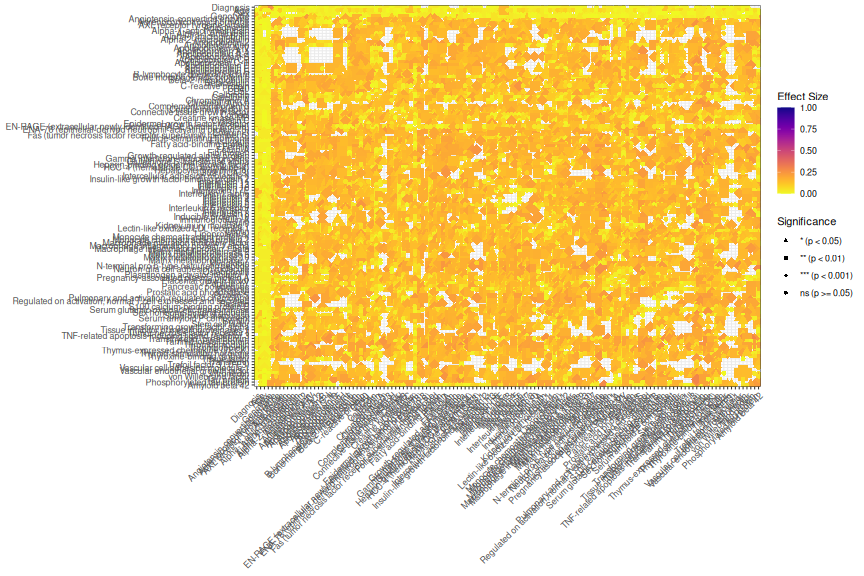

This approach is useful when focusing on a particular biological pathway or clinical domain.

15 Recommended workflow

A common SciDataReportR workflow is:

Use PlotMiningMatrix() to identify potentially interesting relationships.
Review FDR-corrected results.
Identify potential covariates.
Visualize significant findings using plotSigAssociations().
Perform targeted follow-up analyses using:
- MakeComparisonTable()
- PlotCorrelationsHeatmap()
- Regression models
- Longitudinal analyses

16 Summary

PlotMiningMatrix() provides a rapid overview of relationships within a dataset and is particularly useful for exploratory analyses and hypothesis generation.

Key features include:

Automatic test selection
Mixed continuous and categorical variables
Effect size visualization
FDR correction
Identification of candidate covariates
Interactive exploration
Follow-up visualization workflows

18 Session information

sessionInfo()

R version 4.6.1 (2026-06-24)
Platform: x86_64-pc-linux-gnu
Running under: Ubuntu 24.04.4 LTS

Matrix products: default
BLAS:   /usr/lib/x86_64-linux-gnu/openblas-pthread/libblas.so.3
LAPACK: /usr/lib/x86_64-linux-gnu/openblas-pthread/libopenblasp-r0.3.26.so;  LAPACK version 3.12.0

locale:
 [1] LC_CTYPE=C.UTF-8       LC_NUMERIC=C           LC_TIME=C.UTF-8
 [4] LC_COLLATE=C.UTF-8     LC_MONETARY=C.UTF-8    LC_MESSAGES=C.UTF-8
 [7] LC_PAPER=C.UTF-8       LC_NAME=C              LC_ADDRESS=C
[10] LC_TELEPHONE=C         LC_MEASUREMENT=C.UTF-8 LC_IDENTIFICATION=C

time zone: UTC
tzcode source: system (glibc)

attached base packages:
[1] stats     graphics  grDevices utils     datasets  methods   base

other attached packages:
[1] plotly_4.12.0         ggplot2_4.0.3         dplyr_1.2.1
[4] SciDataReportR_20.9.0

loaded via a namespace (and not attached):
 [1] gtable_0.3.6           xfun_0.59              bayestestR_0.18.1
 [4] htmlwidgets_1.6.4      insight_1.5.2          rstatix_1.0.0
 [7] lattice_0.22-9         paletteer_1.7.0        vctrs_0.7.3
[10] tools_4.6.1            generics_0.1.4         datawizard_1.3.1
[13] tibble_3.3.1           pkgconfig_2.0.3        data.table_1.18.4
[16] RColorBrewer_1.1-3     correlation_0.8.8      S7_0.2.2
[19] RcppParallel_5.1.11-2  lifecycle_1.0.5        compiler_4.6.1
[22] farver_2.1.2           snakecase_0.11.1       carData_3.0-6
[25] htmltools_0.5.9        lazyeval_0.2.3         yaml_2.3.12
[28] Formula_1.2-5          pillar_1.11.1          car_3.1-5
[31] tidyr_1.3.2            broom.helpers_1.22.0   viridis_0.6.5
[34] statsExpressions_2.0.0 abind_1.4-8            tidyselect_1.2.1
[37] sjlabelled_1.2.0       digest_0.6.39          mvtnorm_1.4-1
[40] gtsummary_2.5.1        purrr_1.2.2            rematch2_2.1.2
[43] labeling_0.4.3         forcats_1.0.1          ggstatsplot_1.0.0
[46] labelled_2.16.0        fastmap_1.2.0          grid_4.6.1
[49] cli_3.6.6              magrittr_2.0.5         patchwork_1.3.2
[52] utf8_1.2.6             dichromat_2.0-0.1      broom_1.0.13
[55] withr_3.0.3            scales_1.4.0           backports_1.5.1
[58] estimability_2.0.0     httr_1.4.8             rmarkdown_2.31
[61] emmeans_2.0.3          otel_0.2.0             gridExtra_2.3.1
[64] hms_1.1.4              coda_0.19-4.1          evaluate_1.0.5
[67] knitr_1.51             haven_2.5.5            parameters_0.29.2
[70] viridisLite_0.4.3      rstantools_2.6.0       rlang_1.2.0
[73] xtable_1.8-8           glue_1.8.1             jsonlite_2.0.0
[76] effectsize_1.0.2       R6_2.6.1