Screening predictors with MakeUnivariateRegressionTable()

1 Overview

MakeUnivariateRegressionTable() performs large numbers of regression analyses simultaneously and returns publication-ready summary tables.

This approach is particularly useful for:

Biomarker screening
Variable prioritization
Covariate discovery
Exploratory analyses
Hypothesis generation

This vignette demonstrates:

Running multiple univariate regressions
Publication-ready tables
Detailed regression tables
Covariate adjustment
Standardized coefficients
Forest plot visualization

2 Load packages

library(SciDataReportR)
library(dplyr)

3 Load example data

data("SampleData")
data("SampleVariableTypes")

RevaluedObj <- RevalueData(
  SampleData,
  SampleVariableTypes
)

df_Revalued <- RevaluedObj$RevaluedData

4 Define outcomes and predictors

For this example we will evaluate a panel of biomarkers as predictors of several clinical outcomes.

OutcomeVars <- c(
  "Diagnosis",
  "sex"
)

PredictorVars <- c(
  "Genotype",
  "Calbindin",
  "Ferritin",
  "MMP7",
  "Calbindin",
  "Sortilin",
  "Osteopontin"
)

5 Create regression tables

UniObj <- MakeUnivariateRegressionTable(
  data = df_Revalued,
  outcome_vars = OutcomeVars,
  predictor_vars = PredictorVars
)

6 Publication-ready table

The formatted table is designed for reporting and manuscript preparation.

UniObj$FormattedTable

Characteristic	Diagnosis	Sex
Characteristic	OR^1,1,1,1,1,1	OR^1,1,1,1,1,1
Genotype	( )	( )
E2E3	494,242 (624)	0.00 (624)
E2E4	302,597 (624)	0.00 (624)
E3E3	541,490 (624)	0.00 (624)
E3E4	1,336,083 (624)	0.00 (624)
E4E4	3,389,088 (624)	0.00 (624)
Calbindin	1.06 (0.030)	0.91 (0.029)***
Ferritin	1.40 (0.160)*	1.53 (0.149)**
Matrix metalloproteinase 7	1.46 (0.087)***	1.20 (0.074)*
Sortilin	1.65 (0.150)***	0.97 (0.130)
Osteopontin	2.75 (0.326)**	0.63 (0.289)
¹ p<0.05; p<0.01; p<0.001
Abbreviations: CI = Confidence Interval, OR = Odds Ratio, SE = Standard Error

Estimates and standard errors are combined into a compact format and significance stars are automatically added.

7 Detailed regression table

The larger table provides additional model details.

UniObj$LargeTable

Characteristic	Diagnosis			Sex
Characteristic	OR	95% CI	p-value	OR	95% CI	p-value
Genotype
E2E3	494,242	0.00,	0.98	0.00		0.98
E2E4	302,597	0.00,	0.98	0.00		0.98
E3E3	541,490	0.00,	0.98	0.00		0.98
E3E4	1,336,083	0.00,	0.98	0.00		0.98
E4E4	3,389,088	0.00,	0.98	0.00		0.98
Calbindin	1.06	1.00, 1.12	0.071	0.91	0.86, 0.96	<0.001
Ferritin	1.40	1.03, 1.92	0.036	1.53	1.14, 2.06	0.005
Matrix metalloproteinase 7	1.46	1.24, 1.74	<0.001	1.20	1.04, 1.39	0.015
Sortilin	1.65	1.24, 2.23	<0.001	0.97	0.75, 1.26	0.84
Osteopontin	2.75	1.47, 5.28	0.002	0.63	0.36, 1.11	0.11
Abbreviations: CI = Confidence Interval, OR = Odds Ratio

This version is often useful during exploratory analyses and quality control.

8 Including covariates

Covariates can be included in every regression model.

For example, age is commonly included when evaluating biomarker associations.

UniObj_Covar <- MakeUnivariateRegressionTable(
  data = df_Revalued,
  outcome_vars = OutcomeVars,
  predictor_vars = PredictorVars,
  covariates = "age"
)

UniObj_Covar$FormattedTable

Characteristic	Diagnosis	Sex
Characteristic	OR^1,1,1,1,1,1	OR^1,1,1,1,1,1
Genotype	( )	( )
E2E3	577,505 (623)	0.00 (621)
E2E4	369,682 (623)	0.00 (621)
E3E3	676,911 (623)	0.00 (621)
E3E4	1,534,198 (623)	0.00 (621)
E4E4	5,091,058 (623)	0.00 (621)
Calbindin	1.06 (0.030)	0.91 (0.029)***
Ferritin	1.38 (0.162)*	1.55 (0.153)**
Matrix metalloproteinase 7	1.45 (0.088)***	1.18 (0.076)*
Sortilin	1.64 (0.151)**	0.99 (0.133)
Osteopontin	2.69 (0.326)**	0.64 (0.293)
¹ p<0.05; p<0.01; p<0.001
Abbreviations: CI = Confidence Interval, OR = Odds Ratio, SE = Standard Error

This allows investigators to determine whether associations remain significant after accounting for potential confounding factors.

9 Standardized coefficients

When predictors are measured on different scales, standardized coefficients can simplify interpretation.

UniObj_Std <- MakeUnivariateRegressionTable(
  data = df_Revalued,
  outcome_vars = OutcomeVars,
  predictor_vars = PredictorVars,
  Standardize = TRUE
)

UniObj_Std$FormattedTable

Characteristic	Diagnosis	Sex
Characteristic	OR^1,1,1,1,1,1	OR^1,1,1,1,1,1
Genotype	( )	( )
E2E3	494,242 (624)	0.00 (624)
E2E4	302,597 (624)	0.00 (624)
E3E3	541,490 (624)	0.00 (624)
E3E4	1,336,083 (624)	0.00 (624)
E4E4	3,389,088 (624)	0.00 (624)
Calbindin	1.25 (0.125)	0.67 (0.120)***
Ferritin	1.30 (0.126)*	1.39 (0.117)**
Matrix metalloproteinase 7	1.80 (0.135)***	1.33 (0.116)*
Sortilin	1.55 (0.130)***	0.98 (0.113)
Osteopontin	1.49 (0.129)**	0.84 (0.114)
¹ p<0.05; p<0.01; p<0.001
Abbreviations: CI = Confidence Interval, OR = Odds Ratio, SE = Standard Error

Standardized coefficients represent changes in standard deviation units and facilitate comparison across predictors.

10 Accessing model objects

The fitted regression models are returned in the output object.

names(
  UniObj$ModelSummaries
)

[1] "Diagnosis" "sex"

For example:

summary(
  UniObj$ModelSummaries$Diagnosis$Ferritin
)


Call:
stats::glm(formula = f, family = stats::binomial(), data = ModelData)

Coefficients:
            Estimate Std. Error z value Pr(>|z|)
(Intercept)  -1.9184     0.4720  -4.065 4.81e-05 ***
Ferritin      0.3359     0.1601   2.098   0.0359 *
---
Signif. codes:  0 '***' 0.001 '**' 0.01 '*' 0.05 '.' 0.1 ' ' 1

(Dispersion parameter for binomial family taken to be 1)

    Null deviance: 390.60  on 332  degrees of freedom
Residual deviance: 386.11  on 331  degrees of freedom
AIC: 390.11

Number of Fisher Scoring iterations: 4

This allows additional diagnostics and custom analyses.

11 Creating a forest plot

A forest plot provides a compact visual summary of regression results.

ForestPlot <- PlotForestFromTable(
  UniObj
)

ForestPlot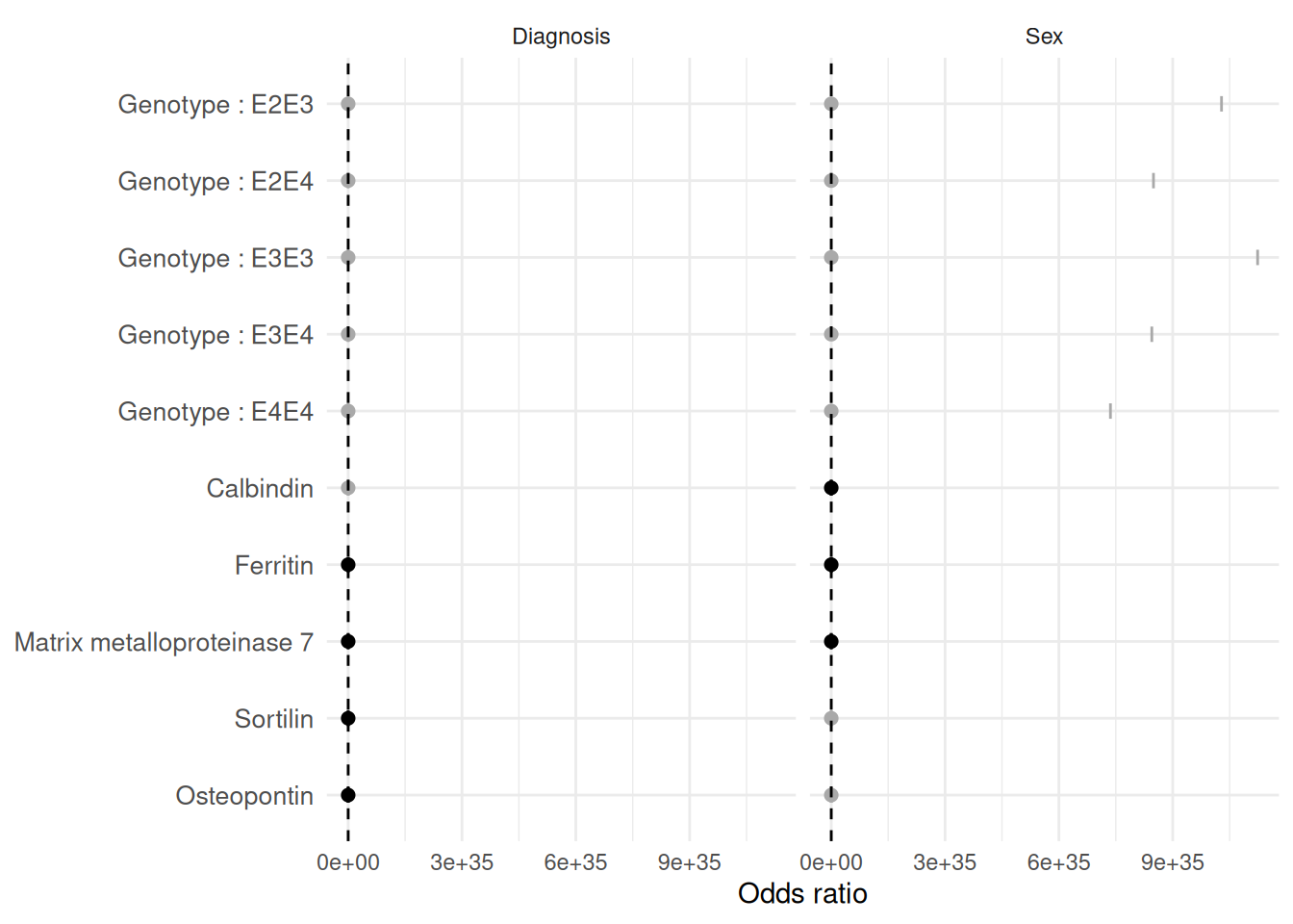

Forest plots make it easy to identify:

Strong predictors
Significant predictors
Direction of effects
Precision of estimates

12 Forest plot with covariate adjustment

The same visualization can be generated using adjusted models.

PlotForestFromTable(
  UniObj_Covar
)

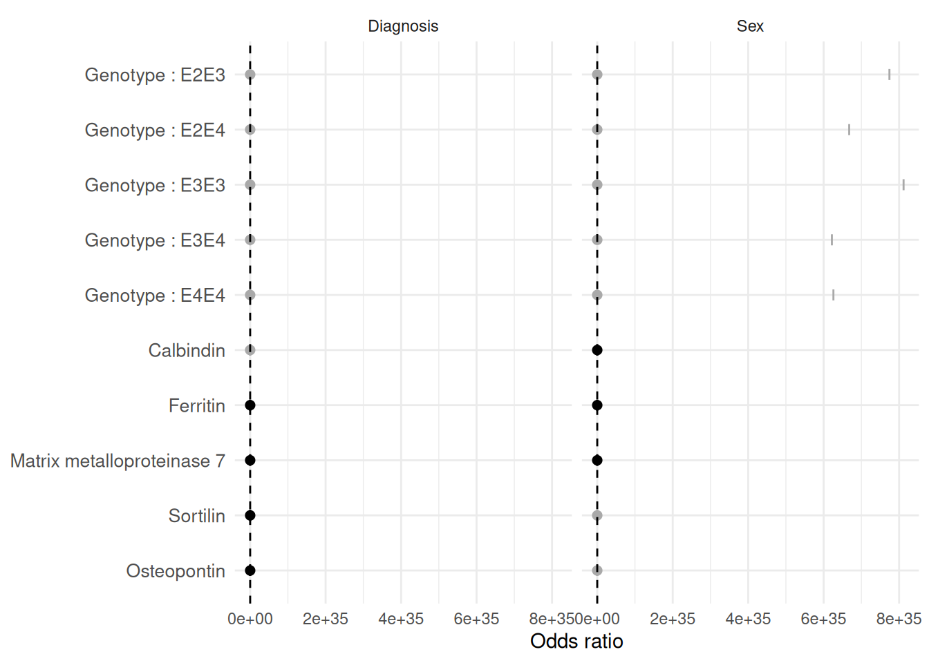
Comparing adjusted and unadjusted models can help identify associations that may be explained by confounding variables.

13 Recommended workflow

A common workflow is:

Use MakeUnivariateRegressionTable() to screen large numbers of predictors.
Review the formatted table.
Compare standardized and unstandardized results.
Add important covariates.
Visualize findings using PlotForestFromTable().
Follow up significant findings using multivariable models.

14 Summary

MakeUnivariateRegressionTable() provides a rapid screening framework for evaluating many predictors across multiple outcomes.

Key features include:

Multiple outcomes
Multiple predictors
Optional covariate adjustment
Standardized coefficients
Publication-ready tables
Detailed regression output
Forest plot visualization

16 Session information

sessionInfo()

R version 4.6.1 (2026-06-24)
Platform: x86_64-pc-linux-gnu
Running under: Ubuntu 24.04.4 LTS

Matrix products: default
BLAS:   /usr/lib/x86_64-linux-gnu/openblas-pthread/libblas.so.3
LAPACK: /usr/lib/x86_64-linux-gnu/openblas-pthread/libopenblasp-r0.3.26.so;  LAPACK version 3.12.0

locale:
 [1] LC_CTYPE=C.UTF-8       LC_NUMERIC=C           LC_TIME=C.UTF-8
 [4] LC_COLLATE=C.UTF-8     LC_MONETARY=C.UTF-8    LC_MESSAGES=C.UTF-8
 [7] LC_PAPER=C.UTF-8       LC_NAME=C              LC_ADDRESS=C
[10] LC_TELEPHONE=C         LC_MEASUREMENT=C.UTF-8 LC_IDENTIFICATION=C

time zone: UTC
tzcode source: system (glibc)

attached base packages:
[1] stats     graphics  grDevices utils     datasets  methods   base

other attached packages:
[1] dplyr_1.2.1           SciDataReportR_20.9.0

loaded via a namespace (and not attached):
 [1] gtable_0.3.6           xfun_0.59              bayestestR_0.18.1
 [4] ggplot2_4.0.3          insight_1.5.2          rstatix_1.0.0
 [7] lattice_0.22-9         paletteer_1.7.0        vctrs_0.7.3
[10] tools_4.6.1            generics_0.1.4         datawizard_1.3.1
[13] tibble_3.3.1           pkgconfig_2.0.3        RColorBrewer_1.1-3
[16] correlation_0.8.8      S7_0.2.2               gt_1.3.0
[19] RcppParallel_5.1.11-2  lifecycle_1.0.5        compiler_4.6.1
[22] farver_2.1.2           stringr_1.6.0          carData_3.0-6
[25] snakecase_0.11.1       litedown_0.9           sass_0.4.10
[28] htmltools_0.5.9        yaml_2.3.12            Formula_1.2-5
[31] pillar_1.11.1          car_3.1-5              tidyr_1.3.2
[34] broom.helpers_1.22.0   statsExpressions_2.0.0 abind_1.4-8
[37] commonmark_2.0.0       tidyselect_1.2.1       sjlabelled_1.2.0
[40] digest_0.6.39          mvtnorm_1.4-1          stringi_1.8.7
[43] gtsummary_2.5.1        purrr_1.2.2            rematch2_2.1.2
[46] labeling_0.4.3         forcats_1.0.1          ggstatsplot_1.0.0
[49] labelled_2.16.0        fastmap_1.2.0          grid_4.6.1
[52] cli_3.6.6              magrittr_2.0.5         base64enc_0.1-6
[55] cards_0.8.0            patchwork_1.3.2        dichromat_2.0-0.1
[58] broom_1.0.13           withr_3.0.3            scales_1.4.0
[61] backports_1.5.1        estimability_2.0.0     rmarkdown_2.31
[64] emmeans_2.0.3          otel_0.2.0             hms_1.1.4
[67] coda_0.19-4.1          evaluate_1.0.5         knitr_1.51
[70] haven_2.5.5            parameters_0.29.2      markdown_2.0
[73] rstantools_2.6.0       rlang_1.2.0            xtable_1.8-8
[76] glue_1.8.1             xml2_1.6.0             jsonlite_2.0.0
[79] effectsize_1.0.2       R6_2.6.1               fs_2.1.0