Univariate Regression Table

Creates a list of univariate regression tables with variable labels and standardized coefficients (if specified).

UnivariateRegressionTable() was renamed to MakeUnivariateRegressionTable() in SciDataReportR 20.5.0 to match the package's Make* naming convention. It remains available as a backwards-compatible synonym.

Usage

MakeUnivariateRegressionTable(
  data,
  outcome_vars,
  predictor_vars,
  covariates = NULL,
  Standardize = FALSE,
  Method = c("auto", "lm", "logistic"),
  LogisticExponentiate = TRUE,
  ReturnModels = FALSE,
  Relabel = TRUE,
  TreatOrdinalAs = "Categorical",
  Data = lifecycle::deprecated(),
  OutcomeVars = lifecycle::deprecated(),
  PredictorVars = lifecycle::deprecated(),
  Covars = lifecycle::deprecated()
)

UnivariateRegressionTable(
  data,
  outcome_vars,
  predictor_vars,
  covariates = NULL,
  Standardize = FALSE,
  Method = c("auto", "lm", "logistic"),
  LogisticExponentiate = TRUE,
  ReturnModels = FALSE,
  Data = lifecycle::deprecated(),
  OutcomeVars = lifecycle::deprecated(),
  PredictorVars = lifecycle::deprecated(),
  Covars = lifecycle::deprecated()
)

Arguments

data

Dataframe containing the variables

outcome_vars

Character vector of outcome variable names

predictor_vars

Character vector of predictor variable names

covariates

Character vector of covariate variable names (default: NULL)

Standardize

Logical indicating whether to standardize numeric variables (default: FALSE)

Method

Character. Regression method to use. "auto" detects linear regression for numeric outcomes and logistic regression for two-level outcomes. "lm" and "logistic" force one model family for all outcomes.

LogisticExponentiate

Logical. If TRUE, logistic regression estimates are exponentiated and reported as odds ratios.

ReturnModels

Logical. If TRUE, return fitted model objects in ModelSummaries. Default is FALSE to keep large screening runs lighter.

Relabel

Logical; if TRUE (default), display attached variable labels.

TreatOrdinalAs

How ordinal outcomes and predictors are handled.

Data

Deprecated (since 19.15.0). Use data instead.

OutcomeVars

Deprecated (since 19.15.0). Use outcome_vars instead.

PredictorVars

Deprecated (since 19.15.0). Use predictor_vars instead.

Covars

Deprecated (since 19.15.0). Use covariates instead.

Value

A list containing:

• FormattedTable: A gt table with formatted regression results

• LargeTable: A gt table with unformatted regression results

• Results: A tidy dataframe with one row per estimated term. Columns: Outcome, OutcomeLabel, OutcomeFamily, EffectType, Predictor, PredictorLabel, Term, Level, TermLabel, N, Estimate, StdError, ConfLow, ConfHigh, PValue, Significant, and ReferenceValue. This dataframe can be filtered and passed directly to PlotForestFromTable().

• ModelSummaries: A list of fitted model objects when ReturnModels = TRUE, otherwise NULL

• Metadata: Outcome families and analysis settings

Details

Fits one model per outcome-predictor pair and collects every result into a single table. "Univariate" means each predictor is tested on its own: for three outcomes and eight predictors this is 24 separate models, not one model with eight terms. That is the screening step - finding which associations exist at all - and it is deliberately different from MultivariableRegressionTable(), which puts all the predictors in one model and reports each one adjusted for the others.

The model family is chosen per outcome. With Method = "auto" (the default), numeric outcomes get linear regression and two-level outcomes get logistic regression, so a mixed set of outcomes can be screened in one call and each is still modeled correctly. "lm" or "logistic" force one family for everything.

Three views of the same results

The return value carries the same estimates in three shapes, for three different jobs:

• FormattedTable - a wide gt table with one spanner per outcome, confidence intervals, stars, and significant results emphasized.

• LargeTable - the same wide layout with the individual model statistics, when the raw numbers matter more than the presentation.

• Results - one tidy row per estimated term, with Estimate, StdError, confidence bounds, PValue, and the labels. This is the one to work with programmatically: filter it, correct it with ApplyFDRCorrection(), or pass it straight to PlotForestFromTable().

Categorical predictors contribute one row per non-reference level, with the level in Level and the level being compared against in ReferenceValue.

Options that change the estimates

Standardize = TRUE z-scores the numeric variables first, so coefficients come back in standard deviations per standard deviation. Use it when predictors are on scales that are not comparable to each other - it is what makes "which predictor matters more" a meaningful question.

covariates adds the named variables to every model, turning a screen of raw associations into a screen of associations adjusted for them. This is usually the difference between "these biomarkers track with the outcome" and "these biomarkers track with the outcome beyond age and sex".

LogisticExponentiate = TRUE (the default) reports logistic results as odds ratios rather than log-odds, so the null value in the table is 1 rather than 0. ReturnModels = TRUE keeps the fitted model objects for residual checks; it is off by default because a large screen would otherwise hold hundreds of models in memory.

Running many models at once means many p-values. Nothing here corrects for that automatically - the family is yours to define - so pass Results$PValue through ApplyFDRCorrection() once you have decided what the family is.

See also

PlotForestFromTable() to visualize Results, MultivariableRegressionTable() for mutually adjusted models, and ApplyFDRCorrection() for multiple-comparison correction.

Examples

# \donttest{
data(SampleData)
data(SampleVariableTypes)

Labelled <- RevalueData(SampleData, SampleVariableTypes)$RevaluedData
# Make the reference example deterministic: age is visibly associated with
# AXL, so the displayed table includes a clear significant result.
ExampleData <- Labelled
set.seed(20260810)
ExampleData$AXL <- as.numeric(scale(ExampleData$age)) * 2 +
  stats::rnorm(nrow(ExampleData), sd = 0.25)
attr(ExampleData$AXL, "label") <- sjlabelled::get_label(Labelled$AXL)

vars_Outcomes <- c("AXL", "tau", "p_tau")
vars_Predictors <- c("age", "sex", "Adiponectin", "Cortisol")

# Three outcomes by four predictors: twelve separate models, one table
urt <- MakeUnivariateRegressionTable(
  data = ExampleData,
  outcome_vars = vars_Outcomes,
  predictor_vars = vars_Predictors
)

# Format 1: the report-ready table
urt$FormattedTable


  

      

        
AXL receptor tyrosine kinase
      
      

        
Tau protein
      
      

        
Phosphorylated tau protein
      
    
Estimate (95% CI)
      
p-value
      
Estimate (95% CI)
      
p-value
      
Estimate (95% CI)
      
p-value
    
Age
0.153 (0.151, 0.155)****
<0.001
-0.000581 (-0.00624, 0.00508)
0.84
0.00212 (-0.00175, 0.006)
0.28
Sex : Male
-0.366 (-0.824, 0.0923)
0.12
-0.0222 (-0.174, 0.129)
0.77
-0.0284 (-0.131, 0.0746)
0.59
Adiponectin
-0.0241 (-0.361, 0.313)
0.89
0.091 (-0.0213, 0.203)
0.11
0.0946 (0.0198, 0.169)*
0.013
Cortisol
0.000744 (-0.0549, 0.0564)
0.98
0.0166 (-0.000439, 0.0336)
0.056
0.0204 (0.00797, 0.0329)**
0.0014

# Format 2: the same results unformatted
urt$LargeTable


  

      

        
AXL receptor tyrosine kinase
      
      

        
Tau protein
      
      

        
Phosphorylated tau protein
      
    
N
      
Estimate
      
SE
      
95% CI Low
      
95% CI High
      
p-value
      
N
      
Estimate
      
SE
      
95% CI Low
      
95% CI High
      
p-value
      
N
      
Estimate
      
SE
      
95% CI Low
      
95% CI High
      
p-value
    
Age
322.000
0.153
0.001
0.151
0.155
0.000
223.000
−0.001
0.003
−0.006
0.005
0.840
322.000
0.002
0.002
−0.002
0.006
0.282
Sex : Male
322.000
−0.366
0.233
−0.824
0.092
0.117
233.000
−0.022
0.077
−0.174
0.129
0.773
333.000
−0.028
0.052
−0.131
0.075
0.588
Adiponectin
322.000
−0.024
0.171
−0.361
0.313
0.888
233.000
0.091
0.057
−0.021
0.203
0.112
333.000
0.095
0.038
0.020
0.169
0.013
Cortisol
322.000
0.001
0.028
−0.055
0.056
0.979
233.000
0.017
0.009
0.000
0.034
0.056
333.000
0.020
0.006
0.008
0.033
0.001

# Format 3: the tidy dataframe, one row per estimated term
htmltools::browsable(htmltools::HTML(as.character(
  FreezeTableHeader(
    dplyr::mutate(
      dplyr::select(
        urt$Results, Outcome, Predictor, TermLabel, Level, N,
        Estimate, StdError, ConfLow, ConfHigh, PValue, Significant
      ),
      dplyr::across(dplyr::where(is.numeric), \(x) signif(x, 3))
    ),
    height = "320px", full_width = TRUE
  )
)))
 Outcome 
   
 Predictor 
   
 TermLabel 
   
 Level 
   
 N 
   
 Estimate 
   
 StdError 
   
 ConfLow 
   
 ConfHigh 
   
 PValue 
   
 Significant 
  
 AXL 
   
 age 
   
 Age 
   
 NA 
   
 322 
   
 0.153000 
   
 0.00109 
   
 0.151000 
   
 0.15500 
   
 0.00000 
   
 TRUE 
  
 AXL 
   
 sex 
   
 Sex : Male 
   
 Male 
   
 322 
   
 -0.366000 
   
 0.23300 
   
 -0.824000 
   
 0.09230 
   
 0.11700 
   
 FALSE 
  
 AXL 
   
 Adiponectin 
   
 Adiponectin 
   
 NA 
   
 322 
   
 -0.024100 
   
 0.17100 
   
 -0.361000 
   
 0.31300 
   
 0.88800 
   
 FALSE 
  
 AXL 
   
 Cortisol 
   
 Cortisol 
   
 NA 
   
 322 
   
 0.000744 
   
 0.02830 
   
 -0.054900 
   
 0.05640 
   
 0.97900 
   
 FALSE 
  
 tau 
   
 age 
   
 Age 
   
 NA 
   
 223 
   
 -0.000581 
   
 0.00287 
   
 -0.006240 
   
 0.00508 
   
 0.84000 
   
 FALSE 
  
 tau 
   
 sex 
   
 Sex : Male 
   
 Male 
   
 233 
   
 -0.022200 
   
 0.07690 
   
 -0.174000 
   
 0.12900 
   
 0.77300 
   
 FALSE 
  
 tau 
   
 Adiponectin 
   
 Adiponectin 
   
 NA 
   
 233 
   
 0.091000 
   
 0.05700 
   
 -0.021300 
   
 0.20300 
   
 0.11200 
   
 FALSE 
  
 tau 
   
 Cortisol 
   
 Cortisol 
   
 NA 
   
 233 
   
 0.016600 
   
 0.00864 
   
 -0.000439 
   
 0.03360 
   
 0.05620 
   
 FALSE 
  
 p_tau 
   
 age 
   
 Age 
   
 NA 
   
 322 
   
 0.002120 
   
 0.00197 
   
 -0.001750 
   
 0.00600 
   
 0.28200 
   
 FALSE 
  
 p_tau 
   
 sex 
   
 Sex : Male 
   
 Male 
   
 333 
   
 -0.028400 
   
 0.05230 
   
 -0.131000 
   
 0.07460 
   
 0.58800 
   
 FALSE 
  
 p_tau 
   
 Adiponectin 
   
 Adiponectin 
   
 NA 
   
 333 
   
 0.094600 
   
 0.03800 
   
 0.019800 
   
 0.16900 
   
 0.01330 
   
 TRUE 
  
 p_tau 
   
 Cortisol 
   
 Cortisol 
   
 NA 
   
 333 
   
 0.020400 
   
 0.00634 
   
 0.007970 
   
 0.03290 
   
 0.00139 
   
 TRUE 
  

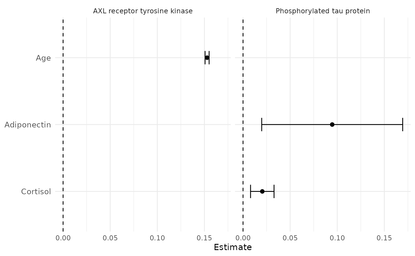
# Filter, correct, and plot
urt$Results$PValueFDR <- ApplyFDRCorrection(urt$Results$PValue)
PlotForestFromTable(urt$Results[urt$Results$PValueFDR < 0.1, ])


# Standardized coefficients, in SD units
MakeUnivariateRegressionTable(
  data = Labelled,
  outcome_vars = vars_Outcomes,
  predictor_vars = vars_Predictors,
  Standardize = TRUE
)$FormattedTable


  

      

        
AXL receptor tyrosine kinase
      
      

        
Tau protein
      
      

        
Phosphorylated tau protein
      
    
Estimate (95% CI)
      
p-value
      
Estimate (95% CI)
      
p-value
      
Estimate (95% CI)
      
p-value
    
Age
0.0957 (-0.0137, 0.205)
0.086
-0.0138 (-0.148, 0.121)
0.84
0.0603 (-0.0498, 0.17)
0.28
Sex : Male
0.0509 (-0.171, 0.272)
0.65
-0.0398 (-0.312, 0.233)
0.77
-0.061 (-0.283, 0.16)
0.59
Adiponectin
0.0806 (-0.0272, 0.188)
0.14
0.109 (-0.0255, 0.243)
0.11
0.135 (0.0284, 0.243)*
0.013
Cortisol
0.129 (0.0219, 0.236)*
0.018
0.118 (-0.00313, 0.24)
0.056
0.175 (0.068, 0.281)**
0.0014

# Every model adjusted for age and sex
MakeUnivariateRegressionTable(
  data = Labelled,
  outcome_vars = vars_Outcomes,
  predictor_vars = c("Adiponectin", "Cortisol", "Ferritin"),
  covariates = c("age", "sex")
)$FormattedTable


  

      

        
AXL receptor tyrosine kinase
      
      

        
Tau protein
      
      

        
Phosphorylated tau protein
      
    
Estimate (95% CI)
      
p-value
      
Estimate (95% CI)
      
p-value
      
Estimate (95% CI)
      
p-value
    
Adiponectin
0.0548 (-0.019, 0.129)
0.14
0.0936 (-0.0231, 0.21)
0.12
0.0924 (0.0158, 0.169)*
0.018
Cortisol
0.0139 (0.00181, 0.0261)*
0.024
0.0164 (-0.000945, 0.0337)
0.064
0.0204 (0.00789, 0.033)**
0.0015
Ferritin
0.326 (0.274, 0.378)****
<0.001
0.348 (0.264, 0.433)****
<0.001
0.29 (0.232, 0.348)****
<0.001

# A binary outcome: logistic regression, reported as odds ratios
urt_Logistic <- MakeUnivariateRegressionTable(
  data = Labelled,
  outcome_vars = "Diagnosis",
  predictor_vars = c("age", "sex", "AXL", "tau", "p_tau")
)
urt_Logistic$Metadata
#> $Outcomes
#>     Outcome OutcomeLabel OutcomeFamily ReferenceLevel EventLevel
#> 1 Diagnosis    Diagnosis      logistic        Control   Impaired
#> 
#> $AnalysisSettings
#> $AnalysisSettings$Method
#> [1] "auto"
#> 
#> $AnalysisSettings$OutcomeVars
#> [1] "Diagnosis"
#> 
#> $AnalysisSettings$PredictorVars
#> [1] "age"   "sex"   "AXL"   "tau"   "p_tau"
#> 
#> $AnalysisSettings$Covars
#> NULL
#> 
#> $AnalysisSettings$Standardize
#> [1] FALSE
#> 
#> $AnalysisSettings$LogisticExponentiate
#> [1] TRUE
#> 
#> $AnalysisSettings$ReturnModels
#> [1] FALSE
#> 
#> 
urt_Logistic$FormattedTable


  

      

        
Diagnosis
      
    
Odds ratio (95% CI)
      
p-value
    
Age
0.994 (0.976, 1.01)
0.55
Sex : Male
1.73 (1.06, 2.82)*
0.028
AXL receptor tyrosine kinase
1.36 (0.794, 2.34)
0.26
Tau protein
7.04 (3.59, 13.8)****
<0.001
Phosphorylated tau protein
6.26 ( 3.4, 11.5)****
<0.001

# Log-odds instead of odds ratios
MakeUnivariateRegressionTable(
  data = Labelled,
  outcome_vars = "Diagnosis",
  predictor_vars = c("age", "AXL", "tau"),
  LogisticExponentiate = FALSE
)$FormattedTable


  

      

        
Diagnosis
      
    
Estimate (95% CI)
      
p-value
    
Age
-0.00558 (-0.024, 0.0129)
0.55
AXL receptor tyrosine kinase
0.31 (-0.231, 0.85)
0.26
Tau protein
1.95 (1.28, 2.62)****
<0.001

# Keep the fitted models for residual checks
urt_Models <- MakeUnivariateRegressionTable(
  data = Labelled,
  outcome_vars = "AXL",
  predictor_vars = c("age", "Cortisol"),
  ReturnModels = TRUE
)
summary(urt_Models$ModelSummaries[[1]])
#>          Length Class Mode
#> age      13     lm    list
#> Cortisol 12     lm    list
# }