Clustering and clinical phenotyping

Raha Dastgheyb

2026-08-18

Purpose

Clinical phenotyping uses prespecified features to discover structure in a training cohort, then places later participants in that fixed phenotype space. Clustering is exploratory: fit indices, internal stability, and clean projection do not establish that a phenotype is biologically real. Clinical interpretation and independent-cohort validation remain essential.

Every pipeline in this package uses the same train-once/project-many contract:

• preprocessing and model parameters are learned from training data only;
• DataWithClusters preserves the original row order and columns;
• incomplete cases remain in the output with NA assignments;
• 80% participant subsample stability refits the entire pipeline, including scaling and PCA/MCA when present;
• fit, membership uncertainty or distance, and projection support are reviewed before phenotypes are named.

method = "exploratory" (or the shorter alias "explore") compares candidate settings and gives an advisory AHP-style recommendation. The researcher then creates an explicit method = "finalize" model for projection.

Lifecycle-specific settings are strict. Exploratory ranges (k_range, models, minPts_range, and epsilon grids) cannot be supplied to a finalized fit; finalized settings (final_k, final_model, final_minPts, and final epsilon) cannot be supplied to exploratory review. This catches calls that would otherwise look valid while silently ignoring part of the request.

Breaking output-name changes

The unreleased clustering interface now uses DataWithClusters rather than df_with_clusters, and ClusterVariableName rather than ClusterName. ModelInfo_MClust is the only correctly cased Mclust-specific field; the erroneous ModelInfo_Mclust field has been removed. complete_rows, CandidateAudit, and internally generated .scidr_rowid columns are no longer public outputs. Use Specification$n_complete for aggregate training support and the fit_table status/warning/error columns to audit candidates.

Every method stores its figures in the same places, so the same review sequence works whichever approach you choose. A figure lives beside the table it summarises rather than in one flat list:

Location	What it shows
fit_plot	candidate solutions across the search grid
ModelInfo$plots	structure of the selected solution
ModelInfo$FitDiagnostics$plots	how individual training cases sit inside that structure
ProbFit$plots	membership confidence
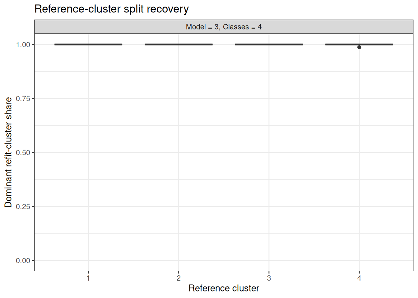
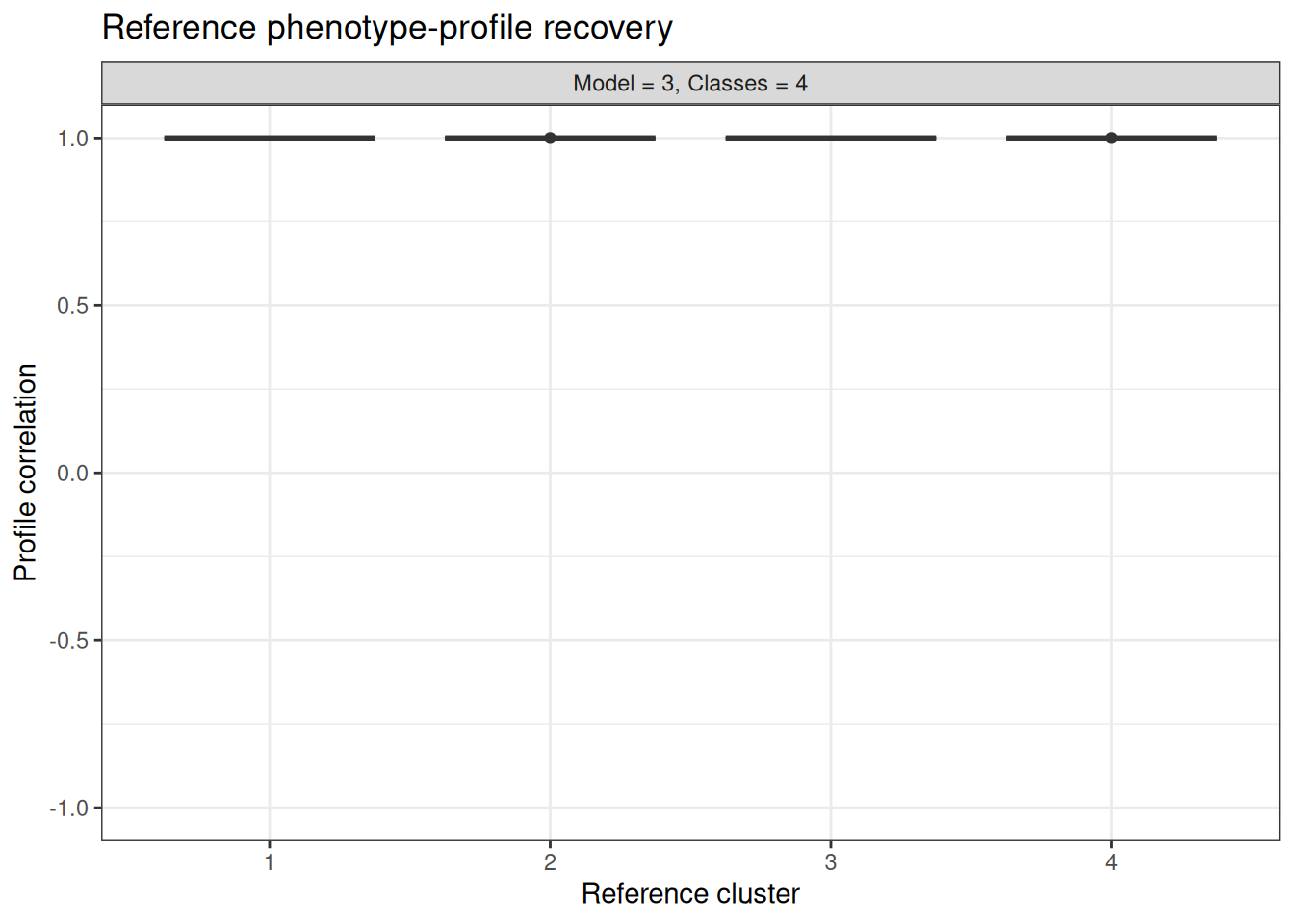
Stability$plots	80% subsample reproducibility
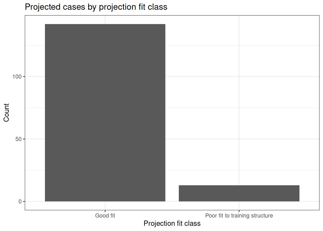
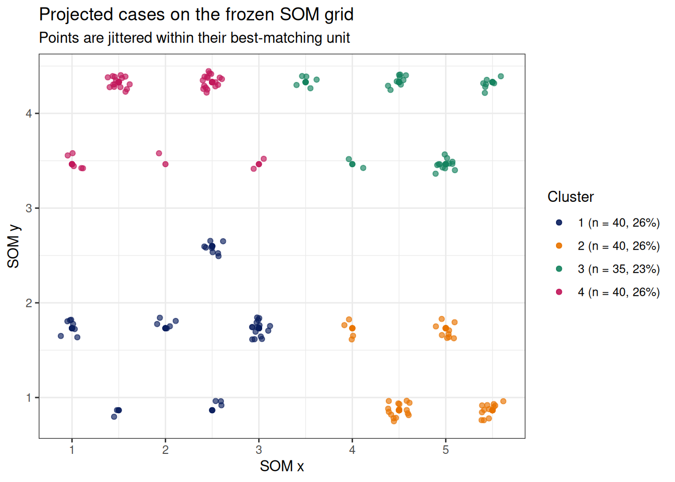
ProjectionFit$plots	projected cases against the frozen training reference

The contents are method-specific: K-means and Gower/PAM give you a silhouette profile, Mclust a BIC curve and an uncertainty map, HDBSCAN a persistence review, LCA item response profiles, and the reduction pipelines a scree plot. The SOM pipeline keeps its own richer set, including the interactive aweSOM maps in ModelInfo_SOM$plots.

Choosing a method

Method	Data and geometry	Primary diagnostics	Projection rule	Ideal situation	Main caveat
SOM + Mclust	Continuous; topology and gradients matter	map fit, posterior, SOM distance, stability	scaling → SOM node → mixture class	phenotype maps and nonlinear gradients	most complex workflow
Mclust	Continuous; Gaussian mixtures	BIC/ICL, entropy, posterior, stability	exact mixture posterior	probabilistic groups with different covariance	sensitive to distributional mismatch
PCA + Mclust	Correlated continuous measures	scree, mixture fit, posterior, stability	frozen PCA → mixture posterior	clustering a lower-dimensional signal space	PCs can obscure individual variables
K-means	Numeric; compact centroid geometry	WSS, silhouette, CH, margin, stability	nearest frozen centroid	simple, interpretable baseline	no probability model
PCA + K-means	Correlated numeric measures	scree, silhouette, distance, stability	frozen PCA → nearest centroid	fast reduced-space baseline	inherits PCA and K-means assumptions
HDBSCAN	Numeric; irregular or unequal-density groups	persistence, membership, noise, support	nearest eligible training core	clusters plus meaningful noise	conservative projection may label many cases noise
Gower + PAM	Mixed numeric/categorical/ordinal	silhouette, medoids, distance, stability	nearest frozen medoid	mixed clinical measures and exemplar participants	coding and variable selection define distance
LCA	Categorical response patterns	BIC, entropy, response probabilities, stability	latent-class posterior	symptom or questionnaire response phenotypes	local-independence assumption
MCA + Mclust	Nominal categorical measures	inertia, mixture fit, posterior, stability	frozen MCA → mixture posterior	reduced categorical response space	MCA dimensions can be abstract

Load the benchmark

Note

The data file is SimulatedPhenotypeData; the codebook is SimulatedPhenotypeVariableTypes. The benchmark contains 320 training and 160 projection participants. TruthCluster, TruthDensityGroup, and Cohort are never supplied to a clustering function. Truth is revealed only as a teaching check after fitting.

The 12 numeric measures are three indicators of each of four independent simulated axes. The default 85% rule therefore retains at least four PCs. Four balanced truth groups use different combinations of these axes. Separate DensityX/DensityY coordinates contain two unequal-density groups and noise; three categorical variables contain deliberately strong class-dependent response patterns. That separation is useful for checking implementation; it is intentionally easier than most real categorical phenotyping problems.

Constructor interface

All clustering constructors use method = "exploratory" to review candidates and method = "finalize" to create a reusable model. Fixed-count methods use k_range and final_k; density methods use minPts_range, epsilon settings, and their matching finalized inputs. Numeric methods use ZScoreType; Scaling is retained as a compatibility alias and must agree if both are supplied.

Workflow	Candidate settings	Finalized settings	Method-specific control
Mclust, PCA + Mclust, MCA + Mclust, SOM + Mclust	k_range, models	final_k, final_model	models: 1 = EEI, 2 = VVI, 3 = EEE
K-means, PCA + K-means, Gower + PAM, latent class	k_range	final_k	nstart for K-means; nrep for LCA
HDBSCAN, SOM + HDBSCAN	minPts_range, epsilon range	final_minPts, final epsilon	extracted class count is data-derived

Continuous workflows

Mclust

Gaussian mixture models provide posterior membership and allow clusters to differ in covariance (Scrucca et al. 2016).

Note

When to use it: continuous measures with approximately mixture-shaped groups. Inspect before naming: BIC/ICL, entropy, posterior confidence, small clusters, subsample ARI/Jaccard, and projected uncertainty.

# A tibble: 9 × 11
  Model ModelName Classes     BIC     ICL Entropy MinClusterN SizeBalance
  <int> <chr>       <int>   <dbl>   <dbl>   <dbl>       <int>       <dbl>
1     1 EEI            10  -5756.  -5771.   0.975           8       0.138
2     1 EEI             9  -5779.  -5793.   0.976           8       0.138
3     1 EEI             8  -5790.  -5803.   0.972          21       0.356
4     1 EEI             7  -5908.  -5923.   0.967          22       0.275
5     1 EEI             6  -5980.  -5995.   0.968          22       0.275
6     1 EEI             4  -6009.  -6009.   1.000          80       1
7     1 EEI             5  -6019.  -6034.   0.967          36       0.45
8     1 EEI             3  -8630.  -8630.   1.000          80       0.5
9     1 EEI             2 -10446. -10446.   0.995          80       0.333
# ℹ 3 more variables: ReproducibilityScore <dbl>, ahp_index <dbl>,
#   Recommended <lgl>

[1] "AHP-style review recommends Gaussian-mixture model (Model = 1, Classes = 4). Review this advisory choice alongside the candidate plots."

K-means

K-means is a useful scaled baseline for compact groups (MacQueen 1967).

Note

When to use it: continuous features with roughly compact, similarly shaped groups. Inspect before naming: WSS, silhouette, Calinski–Harabasz index, centroid distance, assignment margin, and subsample stability.

# A tibble: 9 × 8
  Classes   WSS Silhouette CalinskiHarabasz MinClusterN ReproducibilityScore
    <int> <dbl>      <dbl>            <dbl>       <int>                <dbl>
1       2 2914.      0.272             99.8          80                1
2       3 2073.      0.373            134.           80                0.783
3       4 1264.      0.490            214.           80                1
4       5 1118.      0.453            191.           25                0.871
5       6  977.      0.416            183.           25                0.947
6       7  843.      0.382            185.           25                0.904
7       8  716.      0.345            194.           23                0.937
8       9  668.      0.332            184.           14                0.849
9      10  625.      0.313            177.           14                0.841
# ℹ 2 more variables: ahp_index <dbl>, Recommended <lgl>

[1] "AHP-style review recommends K-means k (Classes = 4). Review this advisory choice alongside the candidate plots."

PCA followed by clustering

PCA concentrates correlated variation into orthogonal dimensions (Jolliffe and Cadima 2016). These pipelines refit scaling and PCA inside every stability 80% subsampling, then use the frozen training transformation for projection.

Note

When to use it: correlated continuous variables where a reduced signal space is clearer than the raw feature space. Inspect before naming: scree plot, retained component count/loadings, downstream fit and stability, score space separation, and projection distance or uncertainty.

# A tibble: 9 × 10
  Model ModelName Classes    BIC    ICL Entropy MinClusterN ReproducibilityScore
  <int> <chr>       <int>  <dbl>  <dbl>   <dbl>       <int>                <dbl>
1     1 EEI             4 -2100. -2100.   1.000          80                1
2     1 EEI             5 -2118. -2150.   0.942          22                0.867
3     1 EEI             6 -2127. -2162.   0.939           5                0.794
4     1 EEI             7 -2141. -2199.   0.906           5                0.631
5     1 EEI             8 -2146. -2219.   0.887           9                0.879
6     1 EEI             9 -2173. -2277.   0.857           9                0.742
7     1 EEI            10 -2200. -2326.   0.836           7                0.687
8     1 EEI             3 -3105. -3106.   0.991          80                1
9     1 EEI             2 -3676. -3720.   0.740          80                1
# ℹ 2 more variables: ahp_index <dbl>, Recommended <lgl>

[1] "AHP-style review recommends PCA plus Gaussian-mixture model (Model = 1, Classes = 4). Review this advisory choice alongside the candidate plots."

[1] 4

# A tibble: 9 × 8
  Classes   WSS Silhouette CalinskiHarabasz MinClusterN ReproducibilityScore
    <int> <dbl>      <dbl>            <dbl>       <int>                <dbl>
1       2  977.      0.282             97.5          80                1
2       3  679.      0.407            139.           80                0.482
3       4  383.      0.543            246.           80                1
4       5  328.      0.513            227.           24                0.884
5       6  277.      0.479            227.           24                0.777
6       7  226.      0.466            242.           24                0.837
7       8  178.      0.444            274.           23                0.939
8       9  162.      0.432            268.           13                0.785
9      10  144.      0.423            270.           13                0.862
# ℹ 2 more variables: ahp_index <dbl>, Recommended <lgl>

[1] "AHP-style review recommends PCA plus K-means k (Classes = 4). Review this advisory choice alongside the candidate plots."

[1] 4

HDBSCAN

HDBSCAN is designed for irregular clusters, unequal density, and noise (McInnes et al. 2017). A projected 0 is an out-of-support/noise assignment, not a new phenotype.

Note

When to use it: density structure is more plausible than centroid geometry and noise is scientifically meaningful. Inspect before naming: persistence, membership, noise burden, outlier scores, stability, and nearest-core support. All-noise candidates are valid negative results.

# A tibble: 6 × 10
  Classes MinPts Epsilon Persistence MeanMembershipProbability NoiseProportion
    <int>  <dbl>   <dbl>       <dbl>                     <dbl>           <dbl>
1       3      6    0           774.                     0.710          0.0688
2       2     10    0          1112.                     0.654          0.134
3       2     14    0           911.                     0.637          0.141
4       3      6    0.05        774.                     0.710          0.0688
5       2     10    0.05       1112.                     0.654          0.134
6       2     14    0.05        911.                     0.637          0.141
# ℹ 4 more variables: MinClusterN <int>, ReproducibilityScore <dbl>,
#   ahp_index <dbl>, Recommended <lgl>

[1] "AHP-style review recommends HDBSCAN density setting (Classes = 2, MinPts = 10, Epsilon = 0.05). Review this advisory choice alongside the candidate plots."

SOM followed by Mclust

Self-organizing maps preserve local topology before mixture clustering (Kohonen 1982).

Note

When to use it: a map of phenotype gradients is as useful as the final labels. Inspect before naming: map topology, quantization/SOM distance, node occupancy, posterior confidence, stability, and projected distance flags.

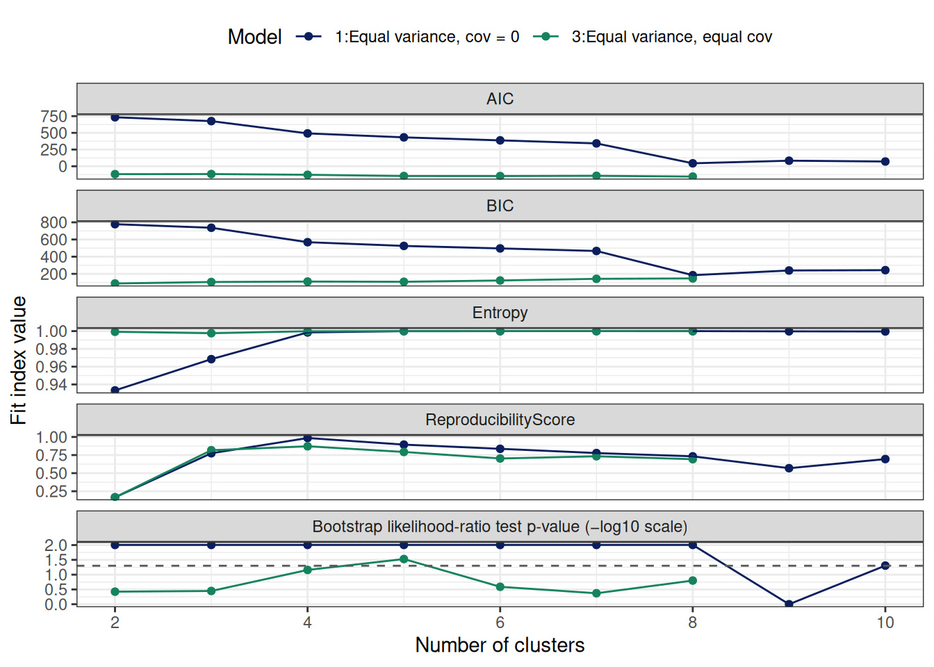
For an analysis, use the complete workflow below. stability_resamples = 30 is a practical internal-stability screen; the rendered vignette uses two resamples only to keep build time reasonable.

data("SimulatedPhenotypeData")

df_Training <- SimulatedPhenotypeData %>% dplyr::filter(Cohort == "Training")
df_Projection <- SimulatedPhenotypeData %>% dplyr::filter(Cohort == "Projection")
vars_Clust <- paste0("Var", 1:12)

Obj_ClustReview <- CreateClusterModel_SOM_MClust(
  df_Training, vars_Clust, k_range = 2:10, models = c(1, 3),
  method = "exploratory"
)
Obj_ClustFinal <- CreateClusterModel_SOM_MClust(
  df_Training, vars_Clust, final_k = 4, final_model = 3,
  method = "finalize", stability_resamples = 30
)
ObjClustProjected <- ProjectCluster(Obj_ClustFinal, df_Projection)

   Model Classes     LogLik parameters  n        AIC       AWE       BIC
1      1       2 -329.58579         37 25  733.17158 1006.5018 778.26998
2      3       2  228.12475        169 25 -118.24949 1136.7320  87.74052
3      1       3 -287.80626         50 25  675.61252 1045.5632 736.55631
4      3       3  240.31502        182 25 -116.63003 1235.0455 105.20537
5      1       4 -182.88068         63 25  491.76135  958.3427 568.55053
6      3       4  258.70221        195 25 -127.40442 1320.9575 110.27637
7      1       5 -140.28938         76 25  432.57876  995.8480 525.21332
8      3       5  280.91625        208 25 -145.83250 1399.2200 107.69367
9      1       6 -104.86298         89 25  387.72596 1047.6860 496.20591
10     3       6  294.29764        221 25 -146.59528 1495.1479 122.77628
11     1       7  -68.97640        102 25  341.95280 1098.6035 466.27814
12     3       7  305.52382        234 25 -143.04764 1595.3863 142.16930
13     1       8   92.86636        115 25   44.26728  897.6087 184.43800
14     3       8  324.17474        247 25 -154.34948 1680.7754 146.71285
15     1       9   86.29563        128 25   83.40875 1033.4415 239.42485
16     1      10  105.45796        141 25   71.08408 1117.8079 242.94557
       CAIC       CLC       KIC     SABIC        ICL   Entropy  prob_min
1  815.2700  661.0382 773.17158  663.5296 -779.13189 0.9332915 0.9301147
2  256.7405 -454.2510  53.75051 -436.3442  -87.74373 0.9992454 0.9996001
3  786.5563  577.5494 728.61252  581.5017 -737.07542 0.9684421 0.9582059
4  287.2054 -478.6348  68.36997 -459.1935 -105.22744 0.9976273 0.9975544
5  631.5505  367.7584 557.76135  373.1817 -568.56586 0.9985197 0.9989606
6  305.2764 -515.4047  70.59558 -494.4367 -110.27761 0.9998412 0.9998736
7  601.2133  282.5787 511.57876  289.5303 -525.21375 0.9999468 0.9999677
8  315.6937 -559.8327  65.16750 -537.3336 -107.69446 0.9999071 0.9999318
9  585.2059  211.7258 479.72596  220.2087 -496.20645 0.9999445 0.9999460
10 343.7763 -586.5953  77.40472 -562.5652 -122.77641 0.9999835 0.9999910
11 568.2781  139.9528 446.95280  149.9667 -466.27815 0.9999983 0.9999985
12 376.1693 -609.0477  93.95236 -583.4864 -142.16948 0.9999800 0.9999596
13 299.4380 -183.7327 162.26728 -172.1877 -184.43800 1.0000000 1.0000000
14 393.7129 -646.3497  95.65052 -619.2571 -146.71397 0.9999090 0.9997218
15 367.4249 -170.5918 214.40875 -157.5150 -239.42880 0.9997308 0.9980997
16 383.9456 -208.9167 215.08408 -194.3085 -242.95179 0.9995963 0.9978376
    prob_max BLRTStatistic BLRTPValue MinProfileNodeN MaxProfileNodeN
1  0.9988990      54.51982 0.00990099               5              20
2  0.9999998      23.21785 0.37623762               4              21
3  0.9994780      83.55906 0.00990099               5              15
4  0.9999982      24.38054 0.35643564               4              17
5  1.0000000     209.85117 0.00990099               5               8
6  1.0000000      36.77438 0.06930693               4               9
7  1.0000000      85.18259 0.00990099               4               7
8  1.0000000      44.42809 0.02970297               3               8
9  1.0000000      70.85280 0.00990099               2               6
10 1.0000000      26.76278 0.25742574               3               6
11 1.0000000      71.77316 0.00990099               2               6
12 1.0000000      22.45236 0.42574257               2               5
13 1.0000000     323.68552 0.00990099               1               5
14 1.0000000      37.30184 0.15841584               2               4
15 1.0000000     -13.14147 1.00000000               1               4
16 1.0000000      38.32467 0.04950495               1               5
   MinProfileNodeProportion MaxProfileNodeProportion StabilitySuccessRate
1                      0.20                     0.80                    1
2                      0.16                     0.84                    1
3                      0.20                     0.60                    1
4                      0.16                     0.68                    1
5                      0.20                     0.32                    1
6                      0.16                     0.36                    1
7                      0.16                     0.28                    1
8                      0.12                     0.32                    1
9                      0.08                     0.24                    1
10                     0.12                     0.24                    1
11                     0.08                     0.24                    1
12                     0.08                     0.20                    1
13                     0.04                     0.20                    1
14                     0.08                     0.16                    1
15                     0.04                     0.16                    1
16                     0.04                     0.20                    1
   StabilityARI_Mean StabilityARI_P05 StabilityJaccard_Mean
1        -0.07945283      -0.08086805             0.4115678
2        -0.07945283      -0.08086805             0.4115678
3         0.72216149       0.48110865             0.8276139
4         0.78077314       0.68890482             0.8531364
5         0.98333461       0.97585943             0.9876529
6         0.85335799       0.78122337             0.8888859
7         0.98310835       0.97546123             0.8054728
8         0.84735613       0.81345926             0.7383310
9         0.94114534       0.90355996             0.7313314
10        0.75392815       0.65675195             0.6512806
11        0.91528914       0.90896571             0.6400826
12        0.82536926       0.82525819             0.6406809
13        0.85784345       0.81953819             0.6067107
14        0.75020911       0.63771710             0.6355237
15        0.66529846       0.65828901             0.4717765
16        0.80725497       0.73087040             0.5819593
   StabilityJaccard_Min ReproducibilityScore AIC_scaled BIC_scaled
1            0.30126050            0.1660575 -1.8609971 -1.9292787
2            0.30126050            0.1660575  0.8299159  0.9543761
3            0.74534161            0.7748877 -1.6790819 -1.7550822
4            0.78699695            0.8169548  0.8247976  0.8814428
5            0.97545732            0.9854938 -1.0980210 -1.0534891
6            0.83368421            0.8711219  0.8588500  0.8602663
7            0.07760141            0.8942906 -0.9109747 -0.8725127
8            0.23595506            0.7928436  0.9170919  0.8710516
9            0.07775769            0.8362384 -0.7692176 -0.7513776
10           0.30804460            0.7026044  0.9195026  0.8080666
11           0.01266026            0.7776858 -0.6245517 -0.6263991
12           0.01803816            0.7330251  0.9082903  0.7270812
13           0.01491228            0.7322771  0.3162822  0.5505669
14           0.02053571            0.6928664  0.9440097  0.7081073
15           0.02439693            0.5685375  0.1925758  0.3209415
16           0.01517857            0.6946071  0.2315279  0.3062390
   Entropy_scaled Reproducibility_scaled   ahp_index
1      -3.3733248           -2.327062909 -2.37266589
2       0.3220404           -2.327062909 -0.05518262
3      -1.4038551            0.324657963 -1.12834032
4       0.2313773            0.507878493  0.61137405
5       0.2813776            1.241939191 -0.15704834
6       0.3554200            0.743800043  0.70458409
7       0.3613381            0.844709625 -0.14435992
8       0.3591120            0.402863759  0.63752983
9       0.3612093            0.591866945 -0.14187972
10      0.3633963            0.009832788  0.52519957
11      0.3642272            0.336845205 -0.13746957
12      0.3631978            0.142328017  0.53522434
13      0.3643198            0.139070131  0.34255977
14      0.3592224           -0.032580477  0.49468976
15      0.3492384           -0.574087113  0.07216715
16      0.3417032           -0.024998753  0.21361782

[1] "AHP (AIC, BIC, Entropy, reproducibility) recommends Model 3 with k = 4 profiles."

# A tibble: 16 × 8
   Model Classes StabilitySuccessRate StabilityARI_Mean StabilityARI_P05
   <int>   <int>                <dbl>             <dbl>            <dbl>
 1     1       2                    1           -0.0795          -0.0809
 2     3       2                    1           -0.0795          -0.0809
 3     1       3                    1            0.722            0.481
 4     3       3                    1            0.781            0.689
 5     1       4                    1            0.983            0.976
 6     3       4                    1            0.853            0.781
 7     1       5                    1            0.983            0.975
 8     3       5                    1            0.847            0.813
 9     1       6                    1            0.941            0.904
10     3       6                    1            0.754            0.657
11     1       7                    1            0.915            0.909
12     3       7                    1            0.825            0.825
13     1       8                    1            0.858            0.820
14     3       8                    1            0.750            0.638
15     1       9                    1            0.665            0.658
16     1      10                    1            0.807            0.731
# ℹ 3 more variables: StabilityJaccard_Mean <dbl>, StabilityJaccard_Min <dbl>,
#   ReproducibilityScore <dbl>

Interpreting a SOM projection

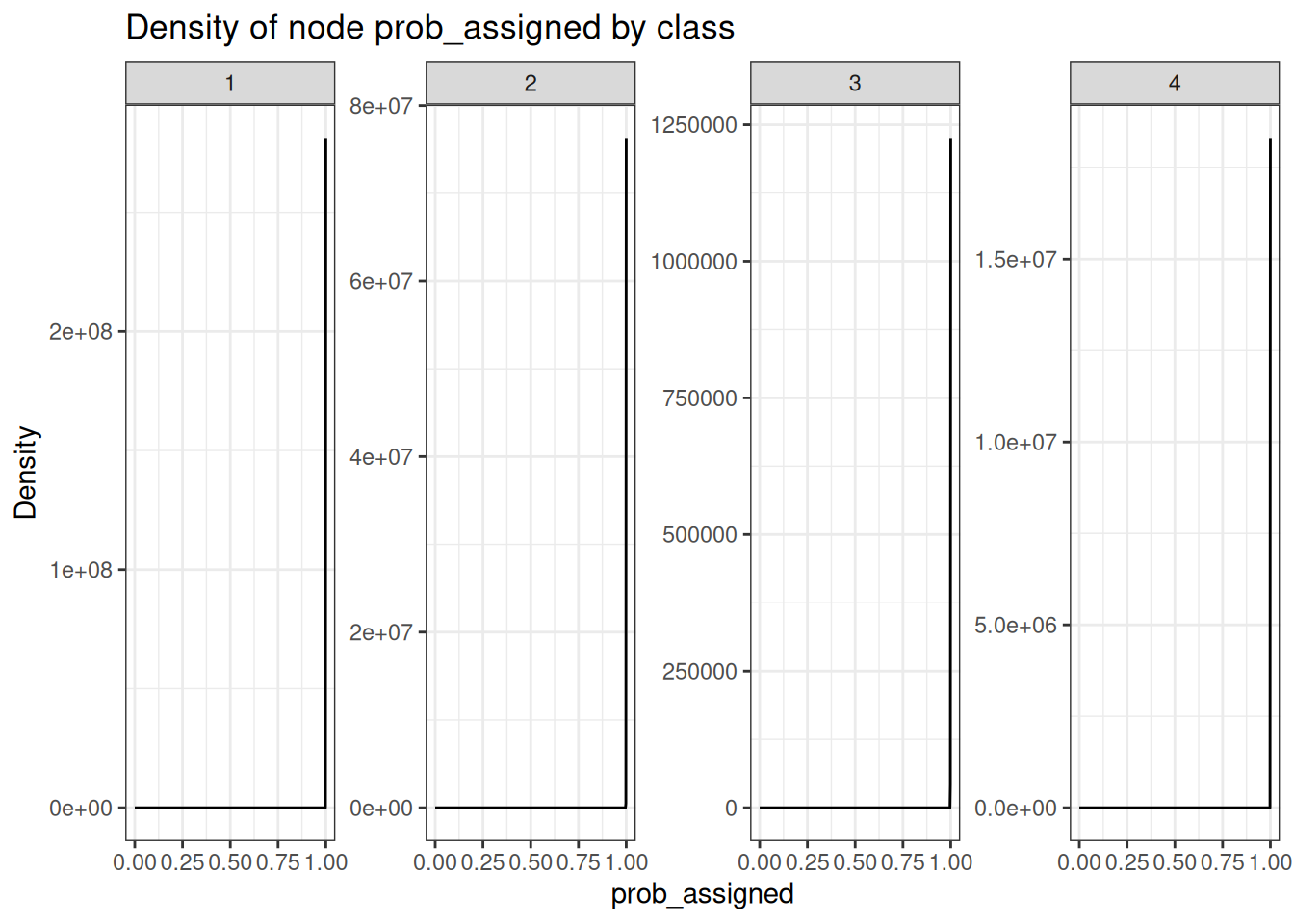
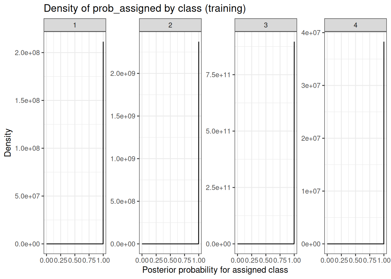
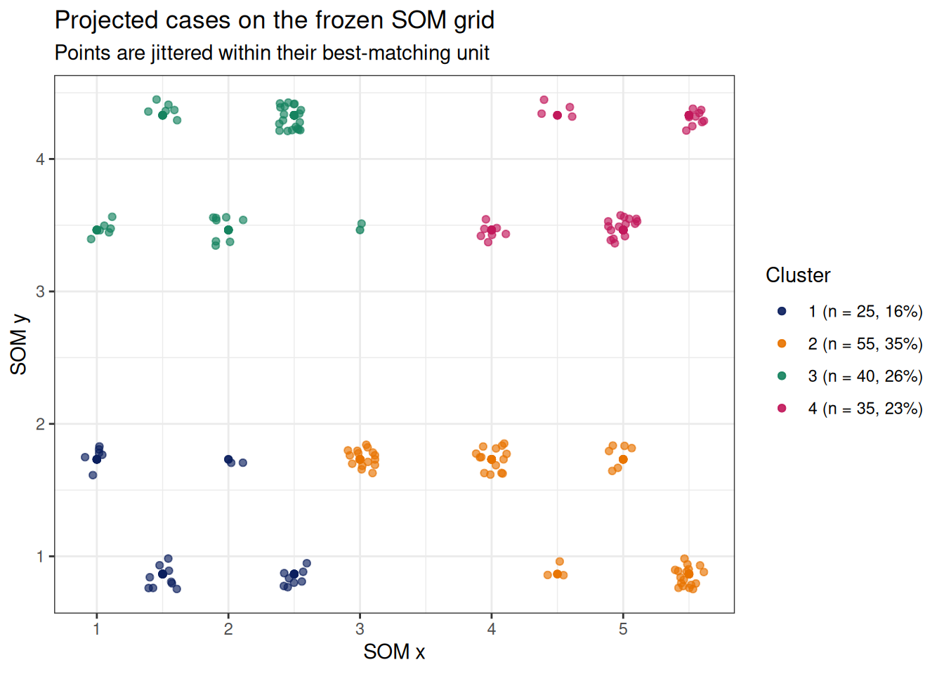
ProbFit answers the assignment question: which cluster was assigned and how certain is the node-derived posterior assignment? Use ProbFit$individual for Cluster, prob_assigned, max_prob, and uncertainty.

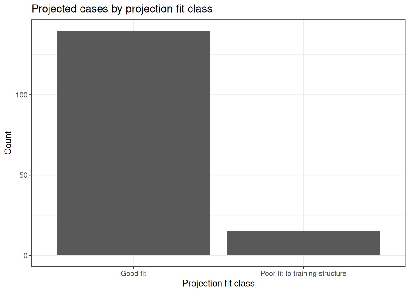
ProjectionFit answers the transportability question: how well do these new participants fit the frozen training SOM? ProjectionFit$individual contains each participant’s best-matching SOM_Node, SOM_Distance, percentile in the training distance distribution, and support flags. A high distance means the participant is less well represented by the training map; it does not by itself invalidate the assigned cluster.

ProjectionFit$out_of_support lists variables with values below the observed training minimum or above the observed training maximum. Projection continues for complete cases, but those values are extrapolations and should be reviewed. ProjectionFit$by_cluster shows whether that concern concentrates in a specific cluster.

ProjectionFit$summary includes node_occupancy_js_divergence, a Jensen–Shannon comparison of the training and projected proportions mapped to each frozen SOM node. A value of zero means identical node occupancy; larger values indicate cohort-level use of a different part of the map. It is not an individual fit score and does not by itself mean the model failed.

Mixed and categorical workflows

Gower distance followed by PAM

Gower distance combines mixed feature types, while PAM represents clusters by observed medoids (Gower 1971; Kaufman and Rousseeuw 1990). Projection uses training ranges, levels, and medoids rather than recalculating them in the new cohort.

Note

When to use it: numeric, binary, ordinal, and nominal measures must be clustered together. Inspect before naming: candidate silhouette, size balance, medoids, numeric and categorical profiles, distance/margin, and subsample stability.

# A tibble: 9 × 8
  Classes Silhouette MeanMedoidDistance MinClusterN SizeBalance
    <int>      <dbl>              <dbl>       <dbl>       <dbl>
1       2      0.260             0.252          119       0.592
2       3      0.485             0.168           84       0.592
3       4      0.752             0.0832          80       1
4       5      0.617             0.0797          29       0.362
5       6      0.485             0.0772          23       0.288
6       7      0.349             0.0748          23       0.288
7       8      0.217             0.0729          16       0.25
8       9      0.192             0.0716          16       0.25
9      10      0.168             0.0703          16       0.25
# ℹ 3 more variables: ReproducibilityScore <dbl>, ahp_index <dbl>,
#   Recommended <lgl>

[1] "AHP-style review recommends Gower/PAM k (Classes = 4). Review this advisory choice alongside the candidate plots."

Latent class analysis

LCA models class-specific categorical response probabilities (Linzer and Lewis 2011).

Note

When to use it: symptom, diagnosis, questionnaire, or assay-call items are the phenotype definition. Inspect before naming: BIC, entropy, class size, response-probability heatmap, posterior confidence, and subsample stability. Low posterior confidence is evidence of weak class separation.

# A tibble: 9 × 9
  Classes   BIC   AIC Entropy MinClassN SizeBalance ReproducibilityScore
    <int> <dbl> <dbl>   <dbl>     <int>       <dbl>                <dbl>
1       4 1328. 1181.   0.999        80      1                     0.971
2       5 1385. 1201.   0.949         3      0.0375                0.993
3       6 1443. 1221.   0.931         2      0.025                 0.961
4       7 1501. 1241.   0.925         2      0.025                 0.838
5       8 1558. 1261.   0.824         2      0.025                 0.841
6       9 1616. 1280.   0.764         2      0.0256                0.900
7       3 1643. 1534.   0.999        80      0.5                   0.988
8      10 1674. 1300.   0.878         1      0.0127                0.917
9       2 1983. 1911.   0.999       160      1                     0.991
# ℹ 2 more variables: ahp_index <dbl>, Recommended <lgl>

[1] "AHP-style review recommends latent class count (Classes = 4). Review this advisory choice alongside the candidate plots."

MCA followed by Mclust

MCA is a dimension-reduction method for nominal categorical measures (Greenacre 2017). Each 80% subsample refits MCA before refitting the mixture.

Note

When to use it: several nominal variables form a useful lower-dimensional category space. Inspect before naming: inertia/scree plot, MCA dimensions, mixture fit, score-space separation, posterior confidence, and stability.

# A tibble: 9 × 11
  Model ModelName Classes    BIC    ICL Entropy MinClusterN SizeBalance
  <int> <chr>       <int>  <dbl>  <dbl>   <dbl>       <int>       <dbl>
1     1 EEI            10  1516.  1516.   1.000           2      0.0263
2     1 EEI             9  1351.  1351.   1.000           3      0.0395
3     1 EEI             8  1057.  1057.   1.000           4      0.0526
4     1 EEI             7   861.   861.   1.000           5      0.0641
5     1 EEI             6   583.   583.   1.000           4      0.05
6     1 EEI             5   400.   400.   1.000           8      0.1
7     1 EEI             4   173.   173.   1.000          80      1
8     1 EEI             3 -1113. -1113.   1.000          80      0.5
9     1 EEI             2 -2486. -2487.   0.991          80      0.333
# ℹ 3 more variables: ReproducibilityScore <dbl>, ahp_index <dbl>,
#   Recommended <lgl>

[1] "AHP-style review recommends MCA plus Gaussian-mixture model (Model = 1, Classes = 4). Review this advisory choice alongside the candidate plots."

Reveal truth for teaching only

The benchmark truth was not used during fitting. ARI is label-invariant, so cluster numbers do not need to match the truth labels. Strong simulation recovery confirms that the examples behave as designed; it is not external or biological validation.

# A tibble: 8 × 3
  Method        TrainingARI ProjectionARI
  <chr>               <dbl>         <dbl>
1 Mclust              1             1
2 K-means             1             1
3 PCA + Mclust        1             1
4 PCA + K-means       1             1
5 Gower + PAM         1             1
6 LCA                 1             0.872
7 MCA + Mclust        1             1
8 SOM + Mclust        0.911         0.785

# A tibble: 2 × 5
  Cohort       ARI NoiseProportion NoiseSensitivity NoiseSpecificity
  <chr>      <dbl>           <dbl>            <dbl>            <dbl>
1 Training   0.841           0.134            0.672                1
2 Projection 0.845           0.125            0.625                1

Compare and interpret profiles

The final label is not the phenotype interpretation. Compare occupancy and feature distributions across plausible models, then use codebook labels when describing the profiles.

  MclustCluster KMeansCluster  n
1             1             1 80
2             2             4 80
3             3             2 80
4             4             3 80

Reproducibility

Candidate metrics and SOM + Mclust workflow

All clustering functions have two modes. method = "exploratory" compares the requested 2:10 candidate settings and returns the fit table, candidate audit, and AHP advisory only. method = "finalize" requires the selected setting and returns assignments, profiles, fit diagnostics, and a reusable projection model. AHP is advisory; its selected row is retained in the table but is never highlighted on a figure.

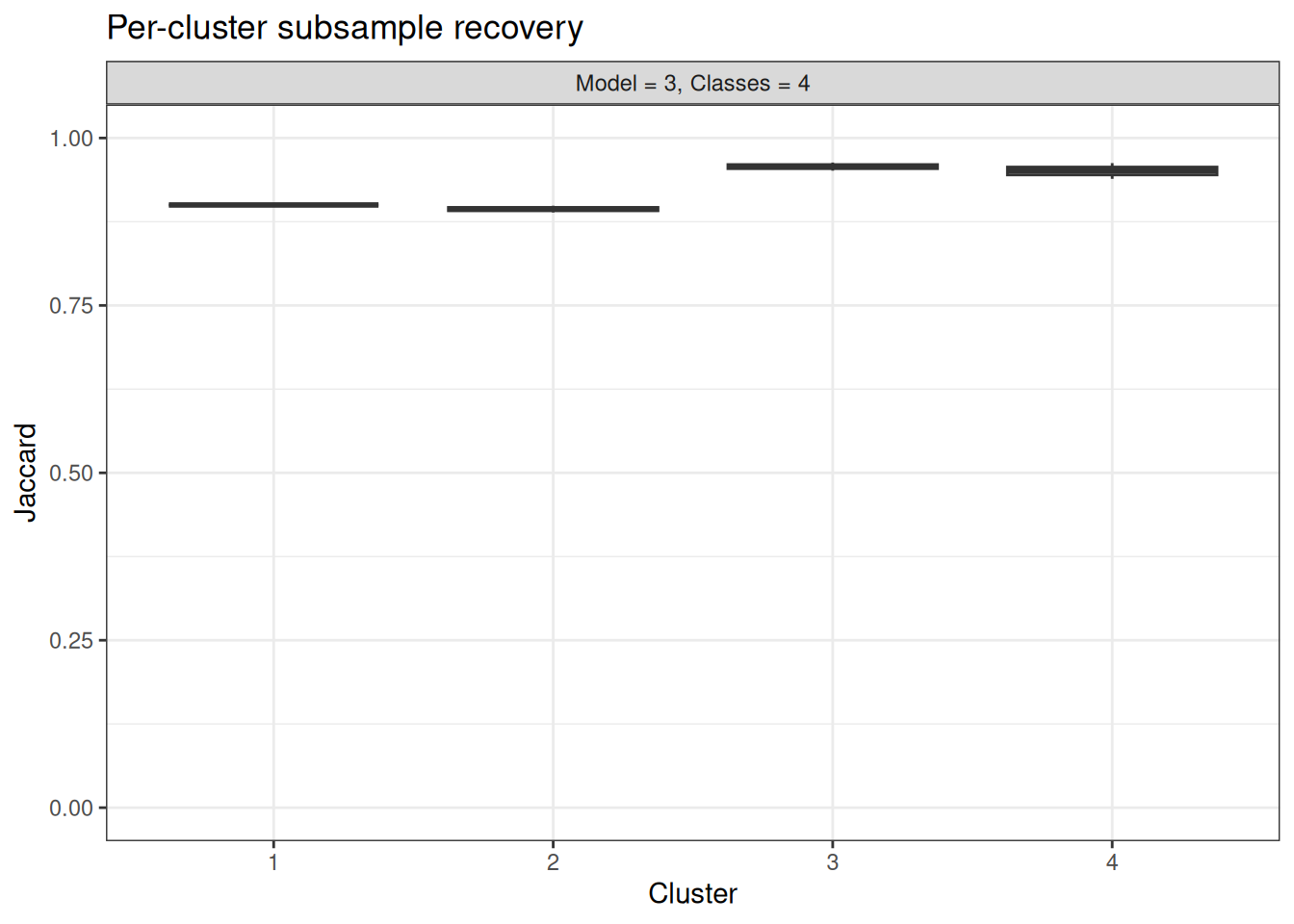
SizeBalance is the smallest extracted cluster/class size divided by the largest (1 is perfectly balanced). MinClusterN/MinClassN is the smallest group size. Subsample ARI measures agreement for the entire partition, whereas per-cluster Jaccard recovery measures whether each reference phenotype reappears after refitting. ReproducibilityScore is the mean of subsample mean ARI and mean Jaccard recovery; subsample success rate is reported separately.

Complementary stability diagnostics

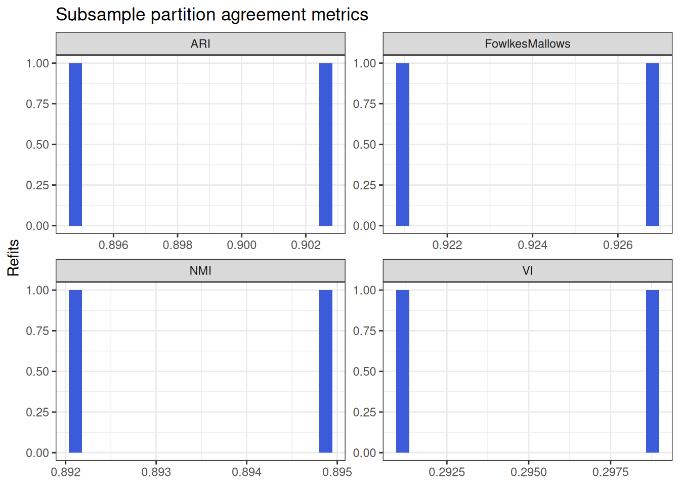
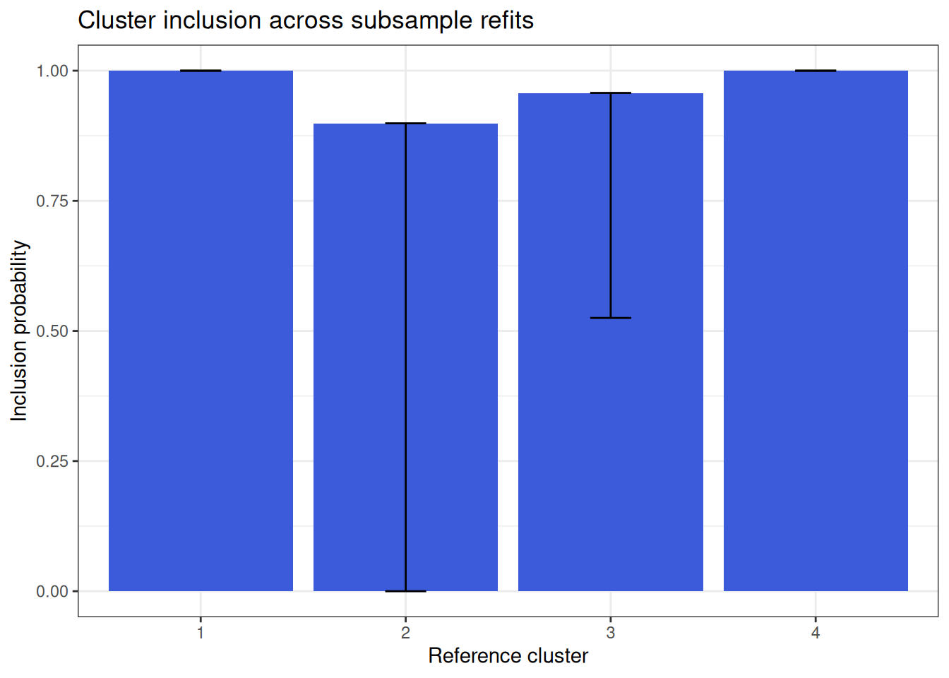
Every successful full-pipeline 80% subsample refit also records variation of information (VI; lower is better), normalized mutual information (NMI; higher is better), and Fowlkes–Mallows agreement (higher is better). These are secondary partition diagnostics: they do not enter ReproducibilityScore or the AHP advisory index. participant_inclusion reports the probability that a participant returns to its reference cluster’s label-matched subsample cluster; cluster_inclusion summarizes that probability by reference cluster.

For complete-case cohorts of 2,000 or fewer participants, coassignment contains the subsample probability that each pair is assigned together and Stability$plots$coassignment displays it. Above that size, the matrix is skipped with a recorded reason to avoid unbounded memory use. For density-based methods, noise remains in global partition metrics but is excluded from inclusion and co-assignment summaries. These diagnostics explain instability; they cannot make a weak phenotype stable.

SOM + Mclust candidate-table fields

CreateClusterModel_SOM_MClust() uses tidyLPA with its mclust backend to fit latent profiles to frozen SOM node codebooks. ShowFitTable() in its help example is only a local display helper: it rounds a table and displays it with a frozen header; it is not a SciDataReportR function.

Field	Definition and interpretation
AIC, AWE, BIC, CAIC, CLC, KIC, SABIC, ICL	Likelihood/information criteria from the LPA fit. Lower values are preferred only when comparing candidates fitted to the same SOM nodes and data. AWE, CLC, and ICL incorporate classification uncertainty (Celeux and Soromenho 1996); KIC is based on symmetric Kullback divergence (Cavanaugh 1999), and SABIC is sample-size adjusted (Sclove 1987). CAIC and CLC are separate criteria, not one combined CAICCLC field.
Entropy	Classification separation summary; higher values indicate cleaner profile separation.
MinProfileNodeN, MaxProfileNodeN	Integer SOM-node counts in the smallest and largest profile.
MinProfileNodeProportion, MaxProfileNodeProportion	The corresponding node counts divided by the total SOM-node count. These replace tidyLPA’s ambiguous decimal n_min and n_max fields.
BLRTStatistic, BLRTPValue	Bootstrap likelihood-ratio statistic and raw p-value for comparing the k-profile fit with k - 1 profiles (Nylund et al. 2007). A small p-value supports the additional profile’s statistical fit, but does not by itself establish stability, clinical meaning, or a final choice; it is unavailable for one profile. The last candidate-review panel displays −log10(BLRTPValue) and marks −log10(0.05), approximately 1.301.
StabilityARI_Mean	Mean adjusted Rand index across successful full-pipeline 80% participant subsample refits without replacement. It may be negative: this means agreement is worse than expected by chance, not an error.
StabilityJaccard_Mean	Mean label-matched, per-profile Jaccard recovery across successful 80% participant subsample refits without replacement.
ReproducibilityScore	Mean of the finite StabilityARI_Mean and StabilityJaccard_Mean; StabilitySuccessRate remains separate.
Reproducibility_scaled	Min-max rescaling of ReproducibilityScore across the current candidate table. It is used only as an AHP input (Akogul and Erisoglu 2017), not as an independently interpretable reproducibility metric.

Method	Candidate metrics
Mclust, PCA + Mclust, MCA + Mclust	BIC/ICL/AIC (information criteria), entropy, maximum posterior uncertainty, minimum cluster size, size balance
K-means, PCA + K-means	WSS, between-cluster sum of squares, silhouette width, Calinski–Harabasz index, minimum size, size balance
Gower + PAM	silhouette width, mean distance to assigned medoid, minimum size, size balance
Latent class	BIC, AIC, log likelihood, entropy, minimum class size, size balance
HDBSCAN and SOM + HDBSCAN	persistence, noise proportion, membership probability, minimum size, size balance; extracted class count is data-derived
SOM + Mclust	LPA AIC/BIC/entropy plus SOM node occupancy and subsample stability

Candidate-metric definitions for every clustering model

All exploratory fit_tables retain the raw metrics produced by their fitted method. AHP is advisory only: any *_scaled field is a within-search rescaling used to construct its index, not a standalone scientific result.

Metric	Definition
Classes	Requested class/cluster count for fixed-count methods. HDBSCAN variants instead report the data-derived number extracted from each density setting.
MinClusterN / MinClassN	Smallest extracted participant cluster/class size. SizeBalance is smallest divided by largest extracted participant group size. SOM + Mclust reports its separate integer node-count and node-proportion fields above.
StabilitySuccessRate	Proportion of requested 80% subsample refits that successfully complete. It is reported separately and is never multiplied into reproducibility.
StabilityARI_Mean, StabilityARI_P05	Mean and fifth percentile of the adjusted Rand index across successful full-pipeline 80% participant subsample refits without replacement (Hubert and Arabie 1985). ARI can be negative when agreement is worse than chance.
StabilityJaccard_Mean, StabilityJaccard_Min	Mean and minimum label-matched per-cluster Jaccard recovery across successful 80% participant subsample refits (Jaccard 1901).
ReproducibilityScore	Mean of finite StabilityARI_Mean and StabilityJaccard_Mean; it is unavailable when neither component is estimable.
AHPIndex / ahp_index and *_scaled	Advisory within-candidate ranking, calculated from the documented method-specific raw metrics. The recommendation does not finalize a model or alter any fit plot.

Pipeline	Method-specific candidate metrics
Mclust, PCA + Mclust, MCA + Mclust	BIC, ICL, AIC, entropy, and maximum posterior uncertainty. BIC and ICL are reported on the scale mclust returns them on, where higher is better (Scrucca et al. 2016); AIC is reported on the conventional scale, where lower is better. Entropy is higher-is-better and uncertainty is lower-is-better.
K-means, PCA + K-means	Within-cluster sum of squares (WSS; lower), between-cluster sum of squares (BSS; higher), mean silhouette width (higher), and Calinski–Harabasz index (higher) (Calinski and Harabasz 1974; Rousseeuw 1987).
Gower + PAM	Mean silhouette width (higher) and mean assigned-medoid Gower distance (lower). The latter is a dissimilarity, not a probability (Gower 1971; Kaufman and Rousseeuw 1990).
Latent class analysis	Log likelihood (higher), AIC/BIC (lower), and entropy (higher) from the fitted item-response model (Linzer and Lewis 2011).
HDBSCAN	Persistence (mean cluster persistence; higher), NoiseProportion (lower), and the data-derived extracted class count. Membership probability and outlier score are assignment diagnostics, not candidate-selection probabilities (McInnes et al. 2017).
SOM + Mclust	The LPA criteria, node allocation, BLRT, and subsample metrics defined in the dedicated SOM + Mclust table below. SOM distances describe map representation, not phenotype probability (Kohonen 1982).
SOM + HDBSCAN	Node-codebook HDBSCAN persistence, noise proportion, extracted node-cluster count, and 80% participant subsample stability. minPts and epsilon are requested settings; class count is data-derived.

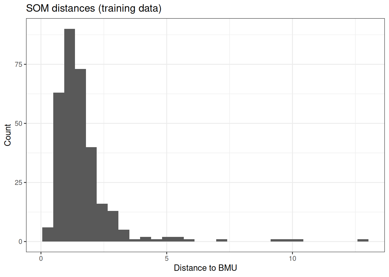
CreateClusterModel_SOM_MClust() is the explicit SOM + Mclust API. CreateSOMClusterModel() remains available for compatibility but is deprecated. The SOM first freezes Z-score preprocessing and learns map nodes; Mclust then clusters those node prototypes. A SOM distance is the distance, in this frozen scaled feature space, between a participant and their best-matching map node. Lower values mean the participant is better represented by the map; they do not mean stronger membership in a phenotype. Interpret it against the frozen training distribution only: distances above the training p95 flag a case that is poorly represented by the training phenotype space.

Specification$rng_kind is R’s RNGkind() configuration: the uniform random number generator, normal random-number generator, and sampling algorithm in effect when the model was fitted. It is provenance for reproducing seeded fits, not a clustering tuning parameter.

How projection works

Every fitted clustering object freezes its preprocessing and records it in Specification; every projected object reports participant-level diagnostics in ProjectionFit$individual, cohort summaries in ProjectionFit$summary, cluster summaries in ProjectionFit$by_cluster, support violations in ProjectionFit$out_of_support, and the applied thresholds in ProjectionFit$policy.

Workflow	Frozen projection rule	Assignment evidence
Mclust	Gaussian-mixture predict() after training scaling	Posterior probabilities and assigned-component Mahalanobis distance
K-means	Nearest frozen centroid	Euclidean centroid distance and second-centroid margin; not a probability
PCA/MCA + clustering	Training scaling and frozen reduction, then the fitted downstream model	The downstream model’s metric/probability
Gower + PAM	Nearest frozen observed medoid using training ranges and levels	Gower medoid distance and runner-up margin
Latent class	Frozen class prevalence and item-response probabilities	Posterior class probabilities
HDBSCAN	Conservative nearest in-training-cluster support rule	Nearest-core distance and support flag; not native HDBSCAN prediction
SOM + Mclust	Frozen scaling, SOM BMU, and node mixture probabilities	BMU distance and node-derived posterior probability
SOM + HDBSCAN	Frozen scaling, SOM BMU, and node HDBSCAN label	BMU distance and inherited node cluster/noise label; not native HDBSCAN prediction

ReproducibilityScore is the mean of subsample mean ARI and mean per-cluster Jaccard recovery. ARI summarizes agreement for the whole partition, whereas Jaccard asks whether each individual phenotype was recovered. Subsample success rate is reported separately and is not folded into the score.

Session information

R version 4.6.1 (2026-06-24)
Platform: x86_64-pc-linux-gnu
Running under: Ubuntu 24.04.4 LTS

Matrix products: default
BLAS:   /usr/lib/x86_64-linux-gnu/openblas-pthread/libblas.so.3
LAPACK: /usr/lib/x86_64-linux-gnu/openblas-pthread/libopenblasp-r0.3.26.so;  LAPACK version 3.12.0

locale:
 [1] LC_CTYPE=C.UTF-8       LC_NUMERIC=C           LC_TIME=C.UTF-8
 [4] LC_COLLATE=C.UTF-8     LC_MONETARY=C.UTF-8    LC_MESSAGES=C.UTF-8
 [7] LC_PAPER=C.UTF-8       LC_NAME=C              LC_ADDRESS=C
[10] LC_TELEPHONE=C         LC_MEASUREMENT=C.UTF-8 LC_IDENTIFICATION=C

time zone: UTC
tzcode source: system (glibc)

attached base packages:
[1] stats     graphics  grDevices utils     datasets  methods   base

other attached packages:
[1] ggplot2_4.0.3         dplyr_1.2.1           SciDataReportR_21.0.0

loaded via a namespace (and not attached):
  [1] RColorBrewer_1.1-3     rstudioapi_0.19.0      jsonlite_2.0.0
  [4] datawizard_1.3.1       correlation_0.8.8      magrittr_2.0.5
  [7] estimability_2.0.0     farver_2.1.2           rmarkdown_2.31
 [10] vctrs_0.7.3            paletteer_1.7.0        CompQuadForm_1.4.4
 [13] base64enc_0.1-6        effectsize_1.0.3       rstatix_1.1.0
 [16] progress_1.2.3         htmltools_0.5.9        forcats_1.0.1
 [19] haven_2.5.5            broom_1.0.13           Formula_1.2-6
 [22] parallelly_1.48.0      htmlwidgets_1.6.4      sandwich_3.1-3
 [25] gsubfn_0.7             plyr_1.8.9             zoo_1.9-0
 [28] emmeans_2.0.4          igraph_2.3.3           mime_0.13
 [31] lifecycle_1.0.5        pkgconfig_2.0.3        Matrix_1.7-5
 [34] sjlabelled_1.2.0       R6_2.6.1               fastmap_1.2.0
 [37] future_1.75.0          shiny_1.14.0           snakecase_0.11.1
 [40] showtext_0.9-8         digest_0.6.39          colorspace_2.1-3
 [43] rematch2_2.1.2         patchwork_1.3.2        irlba_2.3.7
 [46] Hmisc_5.2-6            gtsummary_2.5.1        labeling_0.4.3
 [49] progressr_1.0.0        httr_1.4.8             abind_1.4-8
 [52] compiler_4.6.1         withr_3.0.3            pander_0.6.6
 [55] htmlTable_2.5.0        S7_0.2.2               backports_1.5.1
 [58] viridis_0.6.5          carData_3.0-6          psych_2.6.5
 [61] fastDummies_1.7.6      R.utils_2.13.0         MASS_7.3-65
 [64] scatterplot3d_0.3-45   flashClust_1.1-4       tools_4.6.1
 [67] pbivnorm_0.6.0         MplusAutomation_1.3    foreign_0.8-91
 [70] otel_0.2.0             httpuv_1.6.17          future.apply_1.20.2
 [73] statsExpressions_2.0.0 FactoMineR_2.16        nnet_7.3-20
 [76] R.oo_1.27.1            glue_1.8.1             quadprog_1.5-8
 [79] dbscan_1.2.5           nlme_3.1-169           promises_1.5.0
 [82] gridtext_0.1.6         grid_4.6.1             checkmate_2.3.4
 [85] cluster_2.1.8.2        generics_0.1.4         gtable_0.3.6
 [88] labelled_2.16.0        R.methodsS3_1.8.2      tidyr_1.3.2
 [91] aweSOM_1.3             data.table_1.18.4      hms_1.1.4
 [94] xml2_1.6.0             car_3.1-5              utf8_1.2.6
 [97] ggrepel_0.9.8          RANN_2.6.2             pillar_1.11.1
[100] stringr_1.6.0          later_1.4.8            ggtext_0.1.2
[103] lattice_0.22-9         showtextdb_3.0         ggstatsplot_1.0.0
[106] tidyselect_1.2.1       knitr_1.51             gridExtra_2.3.1
[109] stats4_4.6.1           xfun_0.60              texreg_1.39.5
[112] DT_0.34.0              proto_1.0.0            stringi_1.8.9
[115] yaml_2.3.12            boot_1.3-32            evaluate_1.0.5
[118] codetools_0.2-20       nonnest2_0.5-9         tibble_3.3.1
[121] multcompView_0.1-12    cli_3.6.6              RcppParallel_6.2.0
[124] rpart_4.1.27           xtable_1.8-8           parameters_0.29.2
[127] lavaan_0.7-2           dichromat_2.0-1        Rcpp_1.1.2
[130] tidySEM_0.2.10         globals_0.19.1         coda_0.19-4.1
[133] parallel_4.6.1         kohonen_3.0.13         leaps_3.2
[136] rstantools_2.7.0       prettyunits_1.2.0      mclust_6.1.3
[139] bayestestR_0.18.1      listenv_1.0.0          viridisLite_0.4.3
[142] mvtnorm_1.4-2          sysfonts_0.8.9         scales_1.4.0
[145] crayon_1.5.3           insight_1.5.2          purrr_1.2.2
[148] rlang_1.3.0            mnormt_2.1.2           poLCA_1.6.0.2
[151] tidyLPA_2.0.2         

References

Akogul, Serkan, and Mahir Erisoglu. 2017. “An Approach for Determining the Number of Clusters in a Model-Based Cluster Analysis.” Entropy 19 (9): 452.

Calinski, Tadeusz, and Jerzy Harabasz. 1974. “A Dendrite Method for Cluster Analysis.” Communications in Statistics 3: 1–27.

Cavanaugh, Joseph E. 1999. “A Large-Sample Model Selection Criterion Based on Kullback’s Symmetric Divergence.” Statistical Methodology 61: 165–80.

Celeux, Gilles, and Gilda Soromenho. 1996. “An Entropy Criterion for Assessing the Number of Clusters in a Mixture Model.” Journal of Classification 13: 195–212.

Gower, John C. 1971. “A General Coefficient of Similarity and Some of Its Properties.” Biometrics 27: 857–71.

Greenacre, Michael. 2017. Correspondence Analysis in Practice. 3rd ed. Chapman; Hall/CRC.

Hubert, Lawrence, and Phipps Arabie. 1985. “Comparing Partitions.” Journal of Classification 2: 193–218.

Jaccard, Paul. 1901. “Etude Comparative de La Distribution Florale Dans Une Portion Des Alpes Et Des Jura.” Bulletin de La Société Vaudoise Des Sciences Naturelles 37: 547–79.

Jolliffe, Ian T, and Jorge Cadima. 2016. “Principal Component Analysis: A Review and Recent Developments.” Philosophical Transactions of the Royal Society A 374 (2065): 20150202.

Kaufman, Leonard, and Peter J Rousseeuw. 1990. Finding Groups in Data: An Introduction to Cluster Analysis. Wiley.

Kohonen, Teuvo. 1982. “Self-Organized Formation of Topologically Correct Feature Maps.” Biological Cybernetics 43: 59–69.

Linzer, Drew A, and Jeffrey B Lewis. 2011. “poLCA: An r Package for Polytomous Variable Latent Class Analysis.” Journal of Statistical Software 42 (10): 1–29.

MacQueen, James B. 1967. “Some Methods for Classification and Analysis of Multivariate Observations.” Proceedings of the Fifth Berkeley Symposium on Mathematical Statistics and Probability 1: 281–97.

McInnes, Leland, John Healy, and Steve Astels. 2017. “Hdbscan: Hierarchical Density Based Clustering.” Journal of Open Source Software 2 (11): 205.

Nylund, Karen L, Tihomir Asparouhov, and Bengt O Muthén. 2007. “Deciding on the Number of Classes in Latent Class Analysis and Growth Mixture Modeling: A Monte Carlo Simulation Study.” Structural Equation Modeling 14 (4): 535–69.

Rousseeuw, Peter J. 1987. “Silhouettes: A Graphical Aid to the Interpretation and Validation of Cluster Analysis.” Journal of Computational and Applied Mathematics 20: 53–65.

Sclove, Stanley L. 1987. “Application of Model-Selection Criteria to Some Problems in Multivariate Analysis.” Psychometrika 52: 333–43.

Scrucca, Luca, Michael Fop, Thomas B Murphy, and Adrian E Raftery. 2016. “Mclust 5: Clustering, Classification and Density Estimation Using Gaussian Finite Mixture Models.” Journal of Statistical Software 71 (11): 1–29.