Working with ordinal variables

Why use more than one ordinal perspective?

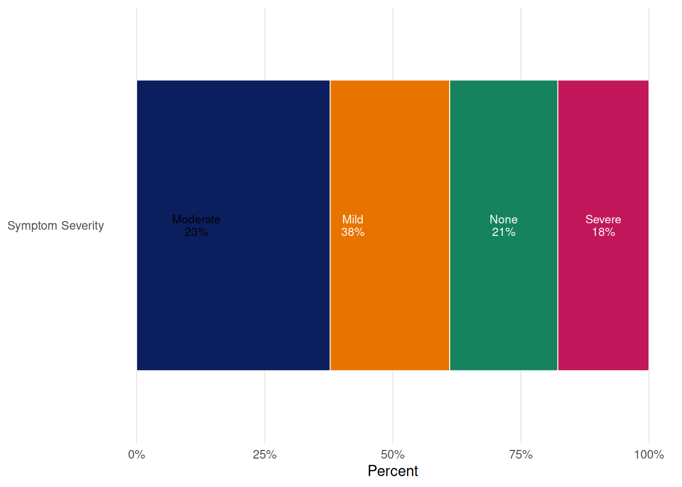
Ordinal variables have a meaningful order, but their adjacent categories are not automatically equally spaced. A symptom scale with None, Mild, Moderate, and Severe can therefore be useful as a categorical outcome when we care about the distribution across levels, or as a continuous score when a one-step increase is a clinically reasonable working scale.

Neither view is universally correct. Looking at both is often useful during EDA: the categorical result shows whether a pattern is concentrated in one level, while the continuous result is a compact summary of an ordered trend. The appropriate confirmatory analysis should still be chosen from the study question, measurement properties, and prespecified analysis plan.

Load packages

Create a labelled ordinal example

Note

This vignette constructs a small example dataset in the document. The VariableTypes object above is the codebook used by RevalueData().

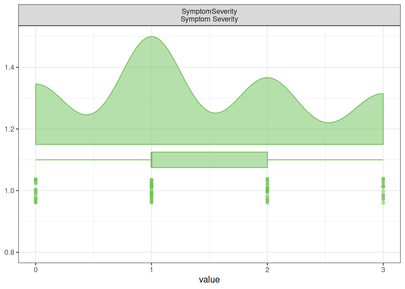
RevalueData() keeps SymptomSeverity as an ordered factor for categorical analysis and records its numeric codebook scores (0 through 3) for a continuous analysis. If a codebook has no complete numeric mapping, the ordered level ranks are used instead.

Comparison tables

TreatOrdinalAs is the common control for tables:

Value	Table behavior
`"Categorical"`	Show ordinal levels and use a categorical test.
`"Continuous"`	Use the preserved numeric score and continuous summary/test.
`"Both"`	Show separate categorical and continuous entries.
`"Exclude"`	Omit ordinal variables from automatic selection.

tbl_Categorical <- MakeComparisonTable(
  data = df_Revalued,
  group_var = "Group",
  variables = "SymptomSeverity",
  TreatOrdinalAs = "Categorical"
)

tbl_Categorical

Comparison by Participant group (values: mean (SD)).
Characteristic	Control N = 45¹	Disease N = 45¹	p-value²	Test²
Symptom Severity			0.00204	Pearson chi-squared
None	14 (31%)	5 (11%)
Mild	20 (44%)	14 (31%)
Moderate	9 (20%)	12 (27%)
Severe	2 (4.4%)	14 (31%)
¹ n (%)
² p-values use Welch t-test (two groups) or ANOVA (more than two groups) for continuous outcomes and chi-square or Fisher’s exact test, selected from expected counts for categorical outcomes.

tbl_Continuous <- MakeComparisonTable(
  data = df_Revalued,
  group_var = "Group",
  variables = "SymptomSeverity",
  TreatOrdinalAs = "Continuous"
)

tbl_Continuous

Comparison by Participant group (values: mean (SD)).
Characteristic	Control N = 45¹	Disease N = 45¹	p-value²	Test²
Symptom Severity	0.98 (0.84)	1.78 (1.02)	<0.001	Welch t-test
¹ Mean (SD)
² p-values use Welch t-test (two groups) or ANOVA (more than two groups) for continuous outcomes and chi-square or Fisher’s exact test, selected from expected counts for categorical outcomes.

tbl_Both <- MakeComparisonTable(
  data = df_Revalued,
  group_var = "Group",
  variables = "SymptomSeverity",
  TreatOrdinalAs = "Both"
)

tbl_Both

Comparison by Participant group (values: mean (SD)).
Characteristic	Control N = 45¹	Disease N = 45¹	p-value²	Test²
Symptom Severity (categorical)			0.00204	Pearson chi-squared
None	14 (31%)	5 (11%)
Mild	20 (44%)	14 (31%)
Moderate	9 (20%)	12 (27%)
Severe	2 (4.4%)	14 (31%)
Symptom Severity (continuous)	0.98 (0.84)	1.78 (1.02)	<0.001	Welch t-test
¹ n (%); Mean (SD)
² p-values use Welch t-test (two groups) or ANOVA (more than two groups) for continuous outcomes and chi-square or Fisher’s exact test, selected from expected counts for categorical outcomes.

With TreatOrdinalAs = "Both", the original data are not changed. The table uses temporary analysis columns and displays them as Symptom Severity (categorical) and Symptom Severity (continuous). With Relabel = FALSE, the same entries use the raw variable name instead: SymptomSeverity (categorical) and SymptomSeverity (continuous).

Plotting options

Plots intentionally allow only representations that make sense for the plot.

Function	Ordinal parameter	Valid values
`PlotCategoricalDistributions()`	`TreatOrdinalAs`	`"Categorical"`, `"Exclude"`
`PlotContinuousDistributions()`	`TreatOrdinalAs`	`"Continuous"`, `"Exclude"`
`PlotCorrelationsHeatmap()`	`TreatOrdinalAs`	`"Continuous"`, `"Exclude"`
`PlotMiningMatrix()`	`TreatOrdinalAs`	all four values

"Both" is rejected by single-representation plots because it would make the analytic question ambiguous. Use separate categorical and continuous plots when you want to inspect both perspectives.

PlotCategoricalDistributions(
  data = df_Revalued,
  variables = "SymptomSeverity",
  TreatOrdinalAs = "Categorical"
)

PlotContinuousDistributions(
  data = df_Revalued,
  variables = "SymptomSeverity",
  TreatOrdinalAs = "Continuous"
)

PlotMiningMatrix() with both representations

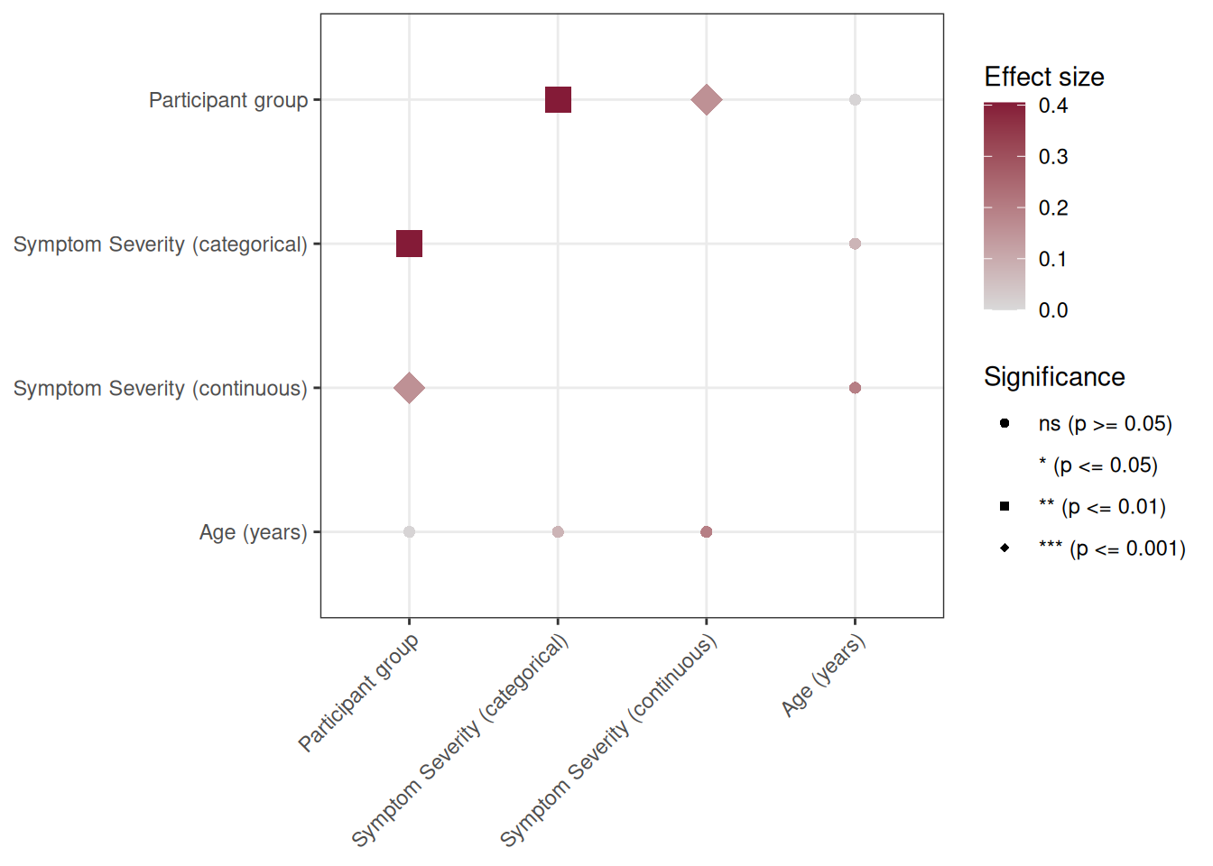
PlotMiningMatrix() is the exception: it can examine mixed variable types, so TreatOrdinalAs = "Both" adds two temporary analysis variables for each ordinal field. It evaluates each representation wherever a valid pairwise test is available; a particular representation will not appear when no compatible variable pair exists.

vars_Mining <- c("Group", "SymptomSeverity", "Age")

MiningObj <- PlotMiningMatrix(
  data = df_Revalued,
  outcome_vars = vars_Mining,
  TreatOrdinalAs = "Both",
  Relabel = TRUE
)

MiningObj$Unadjusted$plot